Copula Modeling for Clinical Trials

Nathan T. James

2019-02-25

Introduction

Background

Randomized clinical trials are considered the gold standard for evaluating a medical intervention and often involve multiple endpoints or outcomes [1,2]. In early phase trials the effect of dose on both efficacy and toxicity endpoints simultaneously is of interest. Similarly, phase III confirmatory trials are often designed to quantify the benefit-risk tradeoffs of a potential treatment. Further, many studies measure the effects of the intervention on a group of several co-primary outcomes representing different dimensions of the underlying disease, and most trials collect data on many types of adverse events. For longitudinal or repeated measures data, measurements of a single outcome variable within a participant over time can be considered multivariate outcomes. In the same way, data from constituent parts of a body system, such as bilateral eye or ear data, are also multivariate. Trials collecting both surrogate and true endpoints offer yet another example. Cluster randomized trials collect data from participants in groups that share a common characteristic such as study center or familial relationship and the dependence within groups is important. The distinguishing trait in all of these situations is that multiple outcomes are observed within a sampling unit so the outcome measures are not independent.

In many of these situations it is common to perform a separate analysis for each outcome, but modeling the multiple outcomes together in a single joint model has several benefits. First, a joint model allows the investigator to answer questions involving combinations of outcomes while accounting for the dependence among them, e.g. “What is the posterior probability that the intervention has a specified level of effectiveness or the risk of adverse events is low?” or “Is the intervention efficacious for three co-primary endpoints simultaneously?” If a Bayesian joint model is used there are additional advantages. Since inference is performed using posterior probabilities, statements involving combinations of the outcomes are more tractable and interpretable. For example, in a trial with three efficacy outcomes it is straightforward to ask about the posterior probability of efficacy – given the observed data and prior – for one outcome, all outcomes, any two outcomes, or some more complex combination (e.g., efficacy for first and either second or third outcome)[3]. Second, dependence may be of interest in its own right. The strength of the relationship between efficacy and safety is central in a benefit-risk analysis. Comparing two drugs with identical efficacy and safety on average, the one with a weaker positive relationship between these outcomes will be preferred since it provides equivalent benefit at lower risk. Understanding the relationship between outcomes through joint modeling provides a more complete picture of how the intervention works in multiple dimensions.

Copulas for Joint Modeling

Several strategies for joint models have been proposed including multivariate normal regression, random effects models, quasi-likelihood/generalized estimating equations (GEE) [4,5] and factorization models [6–9]. However, all of these methods have potential drawbacks. Multivariate normal models are limited by the fact that all the outcomes (or transformations of the outcomes) must be normally distributed. Random effects models such as generalized linear mixed models (GLMM) can deal with non-normal outcomes, but the outcome model parameters have subject-level interpretations which differ from the population-level interpretations that are often of interest. GEE models are incompatible with Bayesian estimation and therefore cannot take advantage of the benefits related to this inferential paradigm. Factorization models – which partition the joint distribution for outcomes \(Y_1\) and \(Y_2\) into conditional and unconditional models \(P(Y_1|Y_2)P(Y_2)\) or \(P(Y_2|Y_1)P(Y_1)\) – treat the two outcomes asymmetrically since one must be chosen for the conditional model and one for the unconditional model and may be complicated to extend to higher dimensions.

This report explores an alternative approach to joint modeling involving multivariate functions called copulas. Copulas allow the investigator to specify the model that is most appropriate for each outcome while also accounting for the relationship between outcomes through a separate dependence model. Crucially, each individual outcome model maintains the same interpretation regardless of the dependence model and the outcome models need not have the same distribution or covariates. This modular approach to specifying the joint model provides increased flexibility and insight into the dependence structure. In many cases, copulas can be considered generalizations or extensions of the other joint modeling approaches.

A copula (denoted \(C\)) is a distribution function that ‘couples’ separate univariate distributions together to create a single joint, multivariate distribution. A \(d\)-dimensional copula combines \(d\) univariate distributions where \(d\) is the number of univariate distributions to be combined. The result is another \(d\)-dimensional multivariate distribution (denoted \(H\)).

As a motivating example, consider two continuous univariate random variables \(Y_1 \sim \text{Normal}(0,1)\) and \(Y_2 \sim \text{Gamma}(4,1)\) perhaps representing efficacy response and adverse event rate, respectively. Figure 1 shows the univariate densities along the top and right margins while the main contour plot shows the level curves of the bivariate density constructed by combining the univariate distributions and a Gumbel copula \(C(u_1, u_2)=\exp[-((-\log u_1)^\theta +(-\log u_2)^\theta)^{1/\theta}]\) with \(\theta=1\frac{1}{3}\) where \(u_1\) and \(u_2\) are values from a uniform distribution on the interval \([0,1]\). The connection between \(u_1\) and \(u_2\) and \(Y_1\) and \(Y_2\) will be explained further in the Copula Models section. Contrast this with Figure 3 which is constructed using identical univariate distributions and a Clayton copula \(C(u_1,u_2)=\max\{u_1^{-\theta} + u_2^{-\theta}-1,0\}^{-1/\theta}\) with \(\theta=\frac{2}{3}\). The values of the copula parameter \(\theta\) were chosen to correspond to Kendall’s \(\tau=0.25\) for both bivariate densities. These plots suggest that the same margins can produce different dependence patterns and the dependence information is contained in the copula and its parameter. Intuitively, this means the interpretation of the margins is the same regardless of the dependence structure. Any analysis which considered each outcome separately would yield identical results under either scenario. For example, \(Pr(\text{efficacy}>0)=0.5\) for both. However, to answer a question related to both outcomes the investigator must account for the dependence structure. The probability of the combined event “\(\text{efficacy}>1\) and \(\text{AE rate}>4\)” is 0.112 for the distribution constructed using the Gumbel copula and 0.094 for the distribution constructed using the Clayton copula.

## Example 1a

# set Kendall's tau
tau <- 0.25

# define Gumbel copula
gc <- gumbelCopula( iTau(gumbelCopula(),tau) )

# define marginal distributions
marg <- c("norm", "gamma")
marg_params <- list(list(mean=0, sd = 1), list(shape=4, rate = 1))

# multivariate distribution combining margins and copula
mvd_gc <- mvdc(copula = gc, margins = marg, paramMargins = marg_params)

# plotting parameters
color2 <- rev(rainbow(11, start = 0/6, end = 4/6))
xl <- c(-4,4)
yl <- c(-0.5,9)

# Gumbel copula
op<-par(fig=c(0,0.75,0,0.75))
gc_comps <- contour(mvd_gc, dMvdc, xlim=xl, ylim=yl, n.grid=50,
      xlab=bquote(Y[1]~~(normal)), ylab=bquote(Y[2]~~('gamma')),
      col=color2, bty="n")

par(fig=c(0,0.75,0.45,1), new=TRUE)
curve(dnorm,xl[1],xl[2],xlab="",ylab="", xlim=xl, bty="n")

par(fig=c(0.6,0.9,0,0.75),new=TRUE)
x_seq<-seq(0,yl[2],length=100)
y_seq<-sapply(x_seq, function(x) dgamma(x,marg_params[[2]]$shape,marg_params[[2]]$rate))
plot(y_seq,x_seq, type="l",xlab="",ylab="",ylim=yl, bty="n")

# scatter plot (NOT shown)
if (0){
par(fig=c(0.6,0.9,0.45,1),new=TRUE)
plot(rMvdc(500, mvd_gc), xlim=xl, ylim=yl, xlab="",ylab="", bty="n",
     pch='.', col=rgb(0,0,0,0.6))
}

# probability of joint event
#P(y1>1,y2>4) = 1- P(y1<1,y2<inf) - P(y1<inf,y2<4) + P(y1<1,y2<4)
#1 - pMvdc(c(1, 1000),mvd_gc) - pMvdc(c(1000, 4),mvd_gc) + pMvdc(c(1, 4),mvd_gc)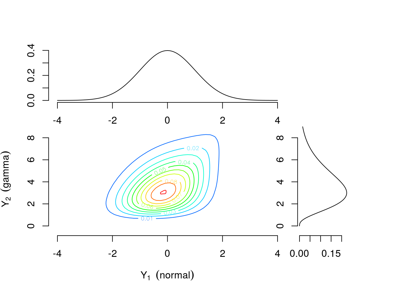

Figure 1: Contour plot of bivariate density with standard normal and gamma(4,1) margins combined using a Gumbel copula with \(\theta=1\frac{1}{3}\)

library(plotly)
# https://plot.ly/r/3d-surface-plots/
# https://plot.ly/r/reference/#surface

# color scheme
num_col <- 100
col_sch <- rev(rainbow(num_col, start = 0/6, end = 4/6))

# contours options
cont_opt <- list(x = list(show=FALSE, usecolormap=FALSE,
                          project=list(x=TRUE,y=FALSE,z=FALSE)),
                 y = list(show=FALSE, usecolormap=FALSE,
                      project=list(x=FALSE,y=TRUE,z=FALSE)) )

#labels and 'camera' angle options
scene_opt <- list( xaxis = list(title = "normal"), yaxis = list(title = "gamma"),
                 zaxis = list(title = "density"),
                 camera = list(eye = list(x = -1.75, y = -1.75, z = 1.25)))

# make plot
# NOTE: need to transpose z matrix output from contour() from to plot correctly
plot_ly(x = gc_comps$x, y = gc_comps$y, z = t(gc_comps$z)) %>%
  add_surface(colors = col_sch, contours = cont_opt) %>%
  layout(scene = scene_opt)

Figure 2: Interactive plot for Figure 1

## Example 1b

# define Clayton copula
cc <- claytonCopula( iTau(claytonCopula(),tau) )

# multivariate distribution combining margins and copula
mvd_cc <- mvdc(copula = cc, margins = marg, paramMargins = marg_params)

# Clayton copula
par(fig=c(0,0.75,0,0.75))
cc_comps <-contour(mvd_cc, dMvdc, xlim=xl, ylim=yl, n.grid=50,
      xlab=bquote(Y[1]~~(normal)), ylab=bquote(Y[2]~~('gamma')),
      col=color2, bty="n")

par(fig=c(0,0.75,0.45,1), new=TRUE)
curve(dnorm,xl[1],xl[2],xlab="",ylab="", xlim=xl, bty="n")

par(fig=c(0.6,0.9,0,0.75),new=TRUE)
x_seq<-seq(0,yl[2],length=100)
y_seq<-sapply(x_seq, function(x) dgamma(x,marg_params[[2]]$shape,marg_params[[2]]$rate))
plot(y_seq,x_seq, type="l",xlab="",ylab="",ylim=yl, bty="n")

# scatter plot (NOT shown)
if (0){
par(fig=c(0.6,0.9,0.45,1),new=TRUE)
plot(rMvdc(500, mvd_cc), xlim=xl, ylim=yl, xlab="",ylab="", bty="n",
     pch='.', col=rgb(0,0,0,0.6))
}

# probability of joint event
#P(y1>1,y2>4) = 1- P(y1<1,y2<inf) - P(y1<inf,y2<4) + P(y1<1,y2<4)
#1 - pMvdc(c(1, 1000),mvd_cc) - pMvdc(c(1000, 4),mvd_cc) + pMvdc(c(1, 4),mvd_cc)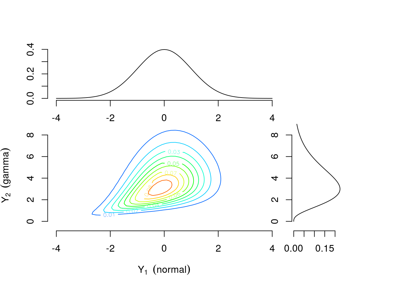

Figure 3: Contour plots of multivariate density with standard normal and gamma(4,1) margins combined using a Clayton copula with \(\theta=\frac{2}{3}\)

# make plot
# NOTE: need to transpose z matrix output from contour() from to plot correctly
plot_ly(x = cc_comps$x, y = cc_comps$y, z = t(cc_comps$z)) %>%
  add_surface(colors = col_sch, contours = cont_opt) %>%
  layout(scene = scene_opt)

Figure 4: Interactive plot for Figure 3

Applications

While there is an extensive literature on copula modeling in fields such as finance, insurance, and meteorology [10–13], applications in clinical trials have been relatively limited compared to other joint modeling approaches described in the previous section. A recent PubMed search for the term “copula” yielded around 700 results compared to over 10,000 results for ‘“GEE” OR “generalized estimating equation”’ and over 30,000 for “random effects”; only 22 results were found for ‘“clinical trial” AND “copula”’. Two illustrative applications are benefit-risk analysis and clustered data.

Costa and Drury [14] considered the use of copula models in joint benefit-risk analysis. The goal is to provide a quantitative display of the tradeoff between efficacy and safety which can be used by investigators, study sponsors, or regulators for decision-making. The inferential framework is Bayesian, so results are presented in terms of the joint posterior probability distribution. Their first simulation study involves a continuous efficacy outcome and a binary safety outcome in a two-arm parallel design. Meester and MacKay [15] used a copula model to analyze data from a randomized clinical trial comparing two antibiotics (cefaclor and amoxicillin) for treatment of otitis media with effusion (OME), an inflammatory disease of the middle ear. Children in the study with either unilateral or bilateral OME were randomly assigned to an antibiotic treatment group and cure status (yes/no) was recorded for each affected ear after two weeks of treatment. The outcomes were either univariate binary, for children with unilateral OME, or bivariate binary, for children with bilateral OME. The investigators were interested in the effect of treatment on cure status after adjusting for age. Both examples are explored in more detail in the Applications section.

References

1. Friedman LM, Furberg CD, DeMets DL, Reboussin DM, Granger CB. Fundamentals of clinical trials. 5th ed. New York, NY: Springer New York; 2015.

2. Evans SR, Ting N. Fundamental concepts for new clinical trialists. Boca Raton: CRC Press, Taylor & Francis Group; 2016.

3. Harrell FE. Musings on multiple endpoints in RCTs. Statistical thinking [Internet]. 2018 [cited 2018 Feb 10];Available from: http://www.fharrell.com/post/ymult/

4. Teixeira-Pinto A, Normand S-LT. Correlated bivariate continuous and binary outcomes: Issues and applications. Statistics in Medicine [Internet] 2009 [cited 2019 Jan 14];28:1753–73. Available from: http://doi.wiley.com/10.1002/sim.3588

5. Leon AR de, Wu B. Copula-based regression models for a bivariate mixed discrete and continuous outcome. Statistics in Medicine [Internet] 2011 [cited 2018 Oct 5];30:175–85. Available from: http://doi.wiley.com/10.1002/sim.4087

6. Catalano PJ, Ryan LM. Bivariate latent variable models for clustered discrete and continuous outcomes. Journal of the American Statistical Association 1992;87:651–8.

9. Olkin I, Tate RF. Multivariate correlation models with mixed discrete and continuous variables. The Annals of Mathematical Statistics [Internet] 1961 [cited 2019 Jan 26];32:448–65. Available from: http://projecteuclid.org/euclid.aoms/1177705052

10. Cherubini U, Luciano E, Vecchiato W. Copula methods in finance. Hoboken, NJ: John Wiley & Sons; 2004.

13. Joe H. Dependence modeling with copulas. Boca Raton: CRC Press, Taylor & Francis Group; 2015.

14. Costa MJ, Drury T. Bayesian joint modelling of benefit and risk in drug development. Pharmaceutical Statistics [Internet] 2018 [cited 2018 Mar 15];Available from: http://doi.wiley.com/10.1002/pst.1852

15. Meester SG, MacKay J. A parametric model for cluster correlated categorical data. Biometrics [Internet] 1994 [cited 2019 Jan 26];50:954–63. Available from: https://www.jstor.org/stable/2533435?origin=crossref