Copula Models
Notation, Definitions, and Sklar’s Theorem
Before defining a copula more rigorously, some results related to univariate probability distributions are reviewed. For a random variable \(Y_1\), the distribution function (or df) \(F_1(y_1)=Pr(Y_1 \le y_1)\). Roughly speaking, this function ‘adds up’ the probability less than or equal to an observed value \(y_1\) of the random variable. All dfs are non-decreasing, right continuous, and satisfy \(\lim_{y_{1} \to -\infty} F_1(y_1)=0\) and \(\lim_{y_{1} \to \infty} F_1(y_1)=1\). When necessary the notation \(F_1(y_1;\mathbf{\gamma}_1)\) will be used to denote the df with parameters \(\mathbf{\gamma}_1\). If \(Y_1\) is a continuous random variable, \(F_1(y_1)=\int_{-\infty}^{y_1}f_1(u)\,du\) where \(f_1(\cdot)\) is the density of \(Y_1\). The inverse of the df is called the quantile function or inverse distribution function and is defined as \(F_1^{-1}(p)=\inf\{y_1:F_1(y_1)\ge p\}\). For a given probability \(p\), the quantile function is the smallest \(y_1\) such that the df evaluated at \(y_1\) is at least as large as \(p\). The df takes real numbers as inputs and returns probabilities while the quantile function takes probabilities and returns real numbers.
A famous result in probability theory called the probability integral transformation says that if the df of a continuous random variable is applied to the random variable itself, the resulting transformed random variable has a continuous standard uniform distribution. So \(F_1(Y_1)=U_1\) where \(U_1 \sim Unif(0,1)\) (see Technical Supplement). This result also implies that the original random variable can be generated given a standard uniform random variable and the quantile function since \(F_{1}^{-1}(U_1)=F_{1}^{-1}(F_1(Y_1))=Y_1\).
When dealing with multivariate outcomes several random variables are involved, so define \(Y_j\) to be the random variable representing the \(j^{th}\) outcome where \(j=1,\ldots,d\) and the dimension, \(d\), is the number of outcomes of interest. In the bivariate case \(d=2\). Let \(F_j\) and \(F_j^{-1}\) be the df and quantile function associated with \(Y_j\), respectively, and \(y_j\) be an observed value of this random variable. Finally, define the multivariate distribution function for the \(Y_j\) to be \(H(\mathbf{y})=Pr(Y_1 \le y_1, \ldots, Y_d \le y_d)\) where \(\mathbf{y} = (y_1,\ldots,y_d)\) is a vector of observed values for \(Y_1\) through \(Y_d\). This function gives the joint probability of being less than or equal to all the observed \(y_j\) simultaneously.
Given a multivariate df \(H\), the individual univariate df \(F_j\) for random variable \(Y_j\) can be recovered by evaluating the limit of \(H\) as all its arguments except for \(y_j\) go to infinity. In the two dimensional case, \(F_1(y_1)=\lim_{y_2 \to \infty}H(y_1,y_2)\) and \(F_2(y_2)=\lim_{y_1 \to \infty}H(y_1,y_2)\). Because of this, the \(F_j\) are often called the marginal dfs. In contrast, given univariate marginal dfs \(F_1,\ldots,F_d\) it is not immediately clear how they relate to \(H\). A foundational 1959 theorem by applied mathematician Abe Sklar [16] provides the answer in the form of an equation that relates the univariate marginal dfs, the copula \(C\), and \(H\). It also guarantees that if the univariate dfs are continuous \(H\) is unique. The same theorem implies the converse: given \(d\) univariate dfs and \(H\), the equation can be used to construct a unique \(C\).
Sklar’s theorem
For a \(d\)-variate distribution \(H\) with \(j=1,\ldots,d\) univariate margins \(F_j\), the copula associated with \(H\) is a distribution function \(C: [0,1]^d \to [0,1]\) with \(Unif(0,1)\) margins that satisfies: \[\begin{equation} H(\mathbf{y})=C(F_1(y_1),\ldots,F_d(y_d)), \, \mathbf{y} \in \mathbb{R}^d \tag{1} \end{equation}\]- If \(H\) is a continuous \(d\)-variate distribution with univariate margins \(F_1,\ldots, F_d\), and corresponding quantile functions \(F_1^{-1},\ldots, F_d^{-1}\), then
\[\begin{equation}
C(\mathbf{u})=H(F_1^{-1}(u_1),\ldots, F_d^{-1}(u_d)),\, \mathbf{u} \in [0,1]^d \tag{2}
\end{equation}\]
is the unique choice.
- If \(H\) is a \(d\)-variate distribution with discrete (or a mix of discrete and continuous) univariate margins, then the copula is unique only on the set \[\begin{equation} Range(F_1) \times \cdots \times Range(F_d) \text{ where } Range(F_j)=\{F_j(x): x \in \mathbb{R}\}\tag{3} \end{equation}\]
Equations (1) and (2) elucidate the link between the marginal dfs \(F_1,\ldots,F_d\) and the joint df \(H\), linked by the copula \(C\). In (1), the probability integral transform ensures that \(F_j(y_j) = u_j\) are observed values from a standard uniform distribution if \(Y_j\) are continuous random variables. If one or more of the marginal dfs are discrete, the copula is only unique on the set defined in equation (3). Informally, the range (also called the image) of a df is the subset of all the numbers to which the function maps. If the dfs are continuous, the range includes all real numbers between 0 and 1, but the output of a discrete df includes only a finite subset of numbers in this interval. So a copula can be constructed with discrete margins, but it is only uniquely defined at certain values. Genest and Nešlehová [17] describe potential problems which can arise when using copulas with discrete margins. For example, the non-uniqueness of \(C\) can lead to identifiability issues in estimation and the dependence between variables is a function of both the copula and the margins, undercutting one of the benefits of copula models. Denuit and Lambert [18] describe restrictions to the range of dependence measures, such as Kendall’s \(\tau\), when the margins are bivariate discrete random variables. Further, the usual probability integral transform does not hold, so more exotic transformations are needed to obtain uniform distributions [19,20]. In many applications, including the two explored in the next section, some of these issues are avoided by positing a latent continuous variable underlying the discrete outcome.
Just as all univariate dfs must satisfy certain properties, each copula must satisfy the following:
- Grounded: \(C(u_1,\ldots, u_d)=0\) if \(u_j=0\) for at least one \(j\)
- Standard Uniform Margins: For any \(j\), \(C(1,\ldots,1,u_j,1,\ldots,1)=u_j\) for all \(u_j \in [0,1]\)
- Non-negative C-volume: For \(d=2\), let \([a_1,a_2] \times [b_1,b_2]\) be a rectangle in the unit square \([0,1]^2\) with lower end point \([a_1,a_2]\) and upper end point \([b_1,b_2]\). The C-volume, \(\Delta_{(\mathbf{a},\mathbf{b}]}C=C(b_1,b_2)-C(b_1,a_2)-C(a_1,b_2)+C(a_1,a_2)\). For a copula, the C-volume must be non-negative for all possible rectangles \([a_1,a_2] \times [b_1,b_2]\). (see Technical Supplement for \(d>2\))
where \(\Phi_2(\cdot|\rho)\) is the bivariate standard normal df with correlation coefficient \(\rho\), \(\Phi^{-1}\) is the quantile function of the univariate standard normal df and \(u_j \in [0,1]\) for \(j=1,2\). If the margins are both standard normal then \(u_1=\Phi(z_1)\) and \(u_2=\Phi(z_2)\) and expression (4) becomes \(C_{\rho}^{Norm}(\Phi(z_1),\Phi(z_2))=\Phi_2(\Phi^{-1}(\Phi(z_1)),\Phi^{-1}(\Phi(z_2))|\rho)=\Phi_2(z_1,z_2|\rho)\) which is the usual bivariate normal df. In other words, a multivariate normal distribution can be represented as a combination of normal margins with a normal copula. This implies that multivariate normal regression models are a special case of normal copula models. Using margins which are not standard normal, however, will produce a distribution that is not multivariate normal. In both scenarios, the dependence between the two margins – contained in the copula – is identical. This is demonstrated in Figure 5 where the same normal copula is used to construct two multivariate dfs (both members of meta-\(C_{R}^{Norm}\) model) by specifying different marginal dfs. Estimates of Spearman’s \(\rho\) and Kendall’s \(\tau\) are similar even though the scatterplots look very different.
## normal copula example
set.seed(2734)

# define normal copula
nc <- normalCopula(0.65)

# multivariate distributions combining margins and copula
mvd_nc1 <- mvdc(copula = nc, margins = c("norm", "norm"),
              paramMargins = list(list(mean = 0, sd = 1),
                                  list(mean = 0, sd = 1)))

mvd_nc2 <- mvdc(copula = nc, margins = c("t", "exp"),
              paramMargins = list(list(df=3),
                                  list(rate = 1)))

if (0){
#calculate true rho and tau
rho(nc); tau(nc)

# plot joint densities
contour(mvd_nc1, dMvdc, xlim=c(-4,4), ylim=c(-4,4),
      xlab="Normal", ylab="Normal")

contour(mvd_nc2, dMvdc, xlim=c(-4,4), ylim=c(-2,6),
      xlab="Student t", ylab="Exponential")
}

#magnify plots
cx <- 1.5

mvd_nc1_samps <- rMvdc(2000, mvd_nc1)
mvd_nc1_rho <- round(cor(mvd_nc1_samps, method="spearman"),3)
mvd_nc1_tau <-round(cor(mvd_nc1_samps, method="kendall"),3)

leg1<-c(as.expression( bquote(hat(rho)~"="~.(mvd_nc1_rho[1,2])) ),
        as.expression( bquote(hat(tau)~"="~.(mvd_nc1_tau[1,2]))))

plot(mvd_nc1_samps, pch=16, col=rgb(0,0,0,0.2), xlab="(1)", ylab="",
     cex=cx, cex.axis=cx, cex.lab=cx)
legend("topleft",legend=leg1, cex=cx)

mvd_nc2_samps <- rMvdc(2000, mvd_nc2)
mvd_nc2_rho <- round(cor(mvd_nc2_samps, method="spearman"),3)
mvd_nc2_tau <- round(cor(mvd_nc2_samps, method="kendall"),3)

leg2<-c(as.expression( bquote(hat(rho)~"="~.(mvd_nc2_rho[1,2])) ),
        as.expression( bquote(hat(tau)~"="~.(mvd_nc2_tau[1,2]))))

plot(mvd_nc2_samps, pch=16, col=rgb(0,0,0,0.1), xlab="(2)", ylab="",
     cex=cx, cex.axis=cx, cex.lab=cx)
legend("topleft",legend=leg2, cex=cx)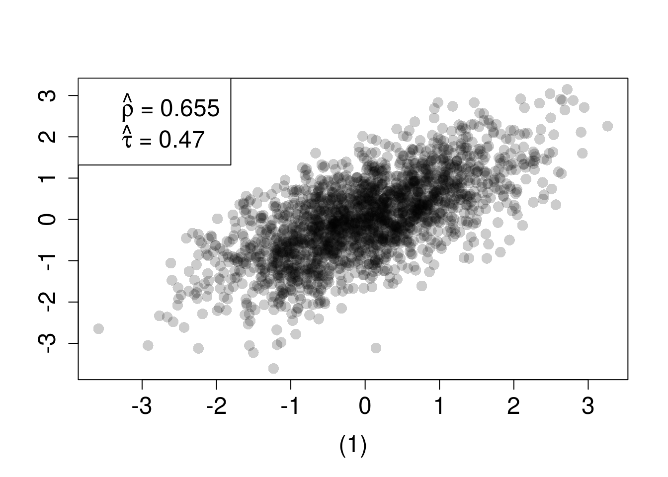
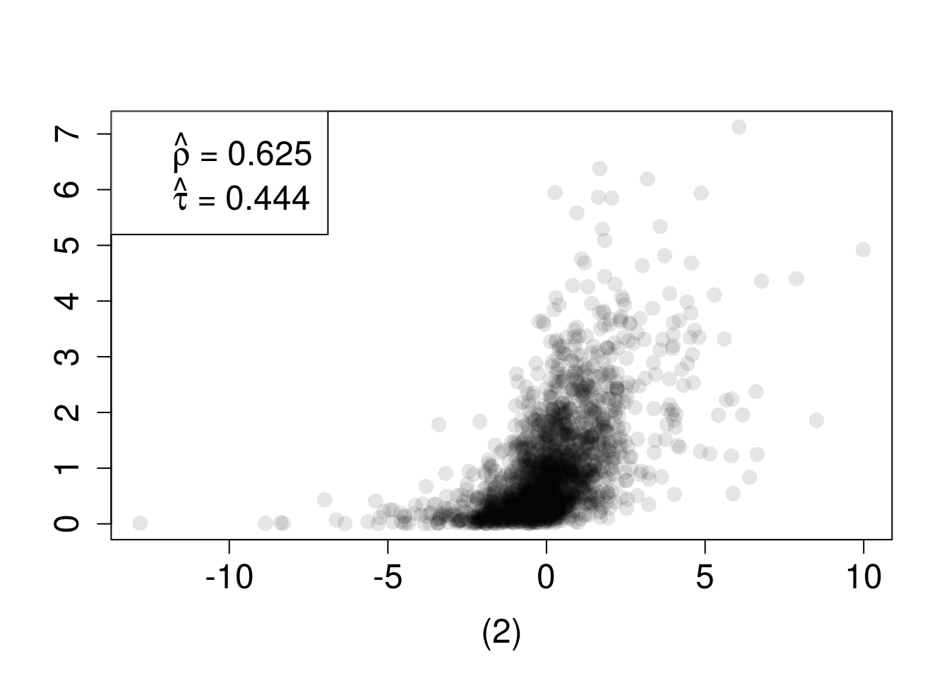
Figure 5: n=2000 random draws from the bivariate distribution constructed with a normal copula and (1) standard normal margins or (2) Student-\(t_3\) and \(exp(1)\) margins. True \(\rho=0.6322\) and \(\tau=0.4505\)
Copula Concepts
Because of its role in tying together univariate dfs, the copula provides a unifying framework to study properties related to association between variables. Many dependency properties can be expressed in terms of copulas and there is a diverse array of copulas available to represent different dependence features.
Independence and Bounds
One of the most important relationships among outcomes is independence or the absence of association, which is defined by the independence copula (also called the product copula) \(\Pi(\mathbf{u})=\prod_{j=1}^{d} u_j, \,\mathbf{u} \in [0,1]^d\). Given continuous random variables \(Y_1\) and \(Y_2\) with unique copula \(C\), \(Y_1\) and \(Y_2\) are independent if and only if \(C=\Pi\). In this case \(H(y_1,y_2)=C(F_1(y_1),F_2(y_2))=\Pi(F_1(y_1),F_2(y_2))=F_1(y_1)F_2(y_2)\).
In addition, limits on dependence can be expressed in terms of copulas by the Fréchet-Hoeffding bounds. For \(\mathbf{u} \in [0,1]^d\), the upper (or comonotonic) bound is \(M(\mathbf{u})=\min\{u_1,\ldots,u_d\}\). \(M\) is itself a copula and defines perfect positive dependence between variables. In this situation, values of all variables increase together almost surely. A simple form of this dependence is a linear relationship between outcomes \(Y_1=a +b Y_2\) with \(b>0\), but many other relationships are also comonotonic. In the case of \(d=2\), the lower (or countermonotonic) bound is \(W(\mathbf{u})=\max\{\sum_{j=1}^{d} u_j -d + 1, 0\}\) and the copula \(W\) defines perfect negative dependence between variables; an increase in the first variable is associated with a decrease in the other variable almost surely. For \(d\ge 3\), \(W\) is not a copula and, in fact, there are no countermonotonic copulas since perfect negative dependence between the first two variables would rule out mutual perfect negative dependence with a third variable. Despite this, \(W\) is still a bound on the values a copula can attain when \(d\ge 3\). Putting these two bounds together, \(W(\mathbf{u}) \le C(\mathbf{u}) \le M(\mathbf{u})\) for any copula \(C\).
# code modified from http://copula.r-forge.r-project.org/book/02_copulas.html

u <- seq(0, 1, length.out = 40) # subdivision points in each dimension
u12 <- expand.grid("u[1]" = u, "u[2]" = u) # build a grid
W <- pmax(u12[,1] + u12[,2] - 1, 0) # values of W on grid
M <- pmin(u12[,1], u12[,2]) # values of M on grid
val.W <- cbind(u12, "W(u[1],u[2])" = W) # append grid
val.M <- cbind(u12, "M(u[1],u[2])" = M) # append grid

cont_opt2 <- list(x = list(show=FALSE, usecolormap=FALSE, highlight=FALSE),
                 y = list(show=FALSE, usecolormap=FALSE, highlight=FALSE),
                 z = list(show=FALSE, usecolormap=FALSE, highlight=FALSE))

scene_opt2 <- list( xaxis = list(title = "u1"), yaxis = list(title = "u2"),
                 zaxis = list(title = ""),
                 camera = list(eye = list(x = -1.75, y = -1.75, z = 1.25)))

# updatemenus component
updatemenus <- list(
  list(
    active = -1,
    type= 'buttons',
    buttons = list(
      list(
        label = "Upper Bound, M",
        method = "update",
        args = list(list(visible = c(FALSE, TRUE)), list(title = "Upper Bound, M"))),
      list(
        label = "Lower Bound, W",
        method = "update",
        args = list(list(visible = c(TRUE, FALSE)), list(title = "Lower Bound, W"))),
      list(
        label = "Both Bounds",
        method = "update",
        args = list(list(visible = c(TRUE, TRUE)), list(title = "Both Bounds"))))
  )
)

plot_ly(x = u, y = u, hoverinfo='none') %>%
  add_surface(z = t(matrix(val.W$`W(u[1],u[2])`,nrow=40, byrow=FALSE)), opacity = 0.75,
              showscale=FALSE, contours = cont_opt2) %>%
  add_surface(z = t(matrix(val.M$`M(u[1],u[2])`,nrow=40, byrow=FALSE)), opacity = 0.65,
              showscale=FALSE, contours = cont_opt2) %>%
  layout(scene = scene_opt2, updatemenus = updatemenus)
Figure 6: Lower and Upper Copula bounds
Invariance
Another important feature of copulas is invariance to monotone increasing transformations. For \((Y_1,\ldots,Y_d) \sim H\) with continuous margins \(F_1,\ldots,F_d\) and copula \(C\) if \(T_j\) is a strictly increasing transformation on \(Range(Y_j)\) then \((T_1(Y_1),\ldots,T_d(Y_d))\) also has copula \(C\). This means that for strictly increasing transformations, as stated by Schweizer and Wolff [21], “the copula is invariant while the margins may be changed at will, it follows that it is precisely the copula which captures those properties of the joint distribution which are invariant under a.s. strictly increasing transformations.” For instance, the copula between \(Y_1\) and \(Y_2\) is the same as the copula between \(\log(Y_1)\) and \(\log(Y_2)\).
Dependence Measures
Many well known measures of association such as Spearman’s \(\rho\), Kendall’s \(\tau\), and the Gini rank correlation coefficient can be expressed in terms of copulas. A conspicuous absence from this list is the most common association measure, the Pearson correlation coefficient, \(r\). While there is a relationship between the copula, its margins and \(r\) in some special cases, Pearson correlation cannot be expressed in terms of the copula alone. Despite the ubiquity of correlation to determine dependence, it is not a good comprehensive measure of association. Unlike the other measures, it only assesses the strength of linear dependence, does not exist for every random vector \((Y_1, Y_2)\), and is not invariant to strictly increasing transformations.
All of these measures summarize the multivariate dependence into a single number meant to convey how strongly ‘large’ values of one variable are associated with ‘large’ values of the other variable. To be more precise, Spearman’s \(\rho\) and Kendall’s \(\tau\) are both measures of concordance. Two independent and identically distributed (iid) pairs \((Y_1,Y_2)\) and \((Y_1',Y_2')\) with joint distribution \(H\), copula \(C\), and common marginal dfs \(F_1\) and \(F_2\), are concordant if \((Y_1-Y_1')(Y_2-Y_2')>0\) and discordant if \((Y_1-Y_1')(Y_2-Y_2')<0\).
The population measure of Kendall’s \(\tau\) is the probability of concordance minus the probability of discordance, so \(\tau=Pr[(Y_1-Y_1')(Y_2-Y_2')>0] - Pr[(Y_1-Y_1')(Y_2-Y_2')<0]\). The same measure can be expressed in terms of the copula \(C\) as \(\tau = 4 \iint_{[0,1]^2} C(u_1,u_2)\, dC(u_1,u_2) - 1\).
The population measure of Spearman’s \(\rho\) can be defined by considering a third pair \((Y_1'',Y_2'')\). The pairs \((Y_1,Y_2)\) and \((Y_1',Y_2'')\) have the same margins, but the first pair has joint distribution \(H\) while the second is independent (since \((Y_1',Y_2')\) and \((Y_1'',Y_2'')\) are iid) so its copula is \(\Pi\). Then \(\rho=3(Pr[(Y_1-Y_1')(Y_2-Y_2'')>0] - Pr[(Y_1-Y_1')(Y_2-Y_2'')<0])\). In terms of copulas, \(\rho=12 \iint_{[0,1]^2}[C(u_1,u_2) -\Pi(u_1,u_2)]\,du_1du_2 = 12\iint_{[0,1]^2}C(u_1,u_2)\,du_1du_2 - 3\). The first equality shows that Spearman’s \(\rho\) is the ‘average’ distance between the distribution of \(Y_1\) and \(Y_2\) (represented by \(C\)) and independence (represented by \(\Pi\)).
Another dependence measure often studied in the context of copulas is tail dependence which quantifies the strength of dependence in the joint tails of the multivariate distribution. Multivariate dfs with ‘heavier’ tails place higher probability on extreme events occuring simultaneously. Figure 7 (reproduced using code from [22]) shows four samples from a Fréchet class with identical margins and Kendall’s \(\tau\), but different copulas. The differences in the proportion of samples in the bivariate tails provides some insight into the concept of tail dependence. The normal copula has no tail dependence (unless the variables are comonotonic), while the Student-\(t\) has symmetric upper and lower tail dependence. The Gumbel copula only allows upper tail dependence and the Clayton copula only allows lower tail dependence.
The lower tail dependence parameter is formally defined as \(\lambda_l = \lambda_l(Y_1,Y_2)= \lim_{q\downarrow 0} Pr(Y_2 \le F_{2}^{-1}(q)|Y_1 \le F_{1}^{-1}(q))\), i.e., the limit as \(q\) goes to 0 of the conditional probability of \(Y_2\) being smaller than the \(q^{th}\) quantile given that \(Y_1\) is smaller than the \(q^{th}\) quantile. In terms of the copula between \((Y_1,Y_2)\), \(\lambda_l(C)=\lim_{q\downarrow 0}\frac{C(q,q)}{q}\). If \(\lambda_l \in (0,1]\), then \(Y_1\) and \(Y_2\) are lower tail dependent. Similarly, upper tail dependence is defined as \(\lambda_u=\lim_{q\uparrow 1} Pr(Y_2 > F_{2}^{-1}(q)|Y_1 > F_{1}^{-1}(q))=\lim_{q\uparrow 1} \frac{1-2q + C(q,q)}{1-q}\). If \(\lambda_u \in (0,1]\), then \(Y_1\) and \(Y_2\) are upper tail dependent.
### Tail Dependence
## Four distributions with N(0,1) margins and a Kendall's tau of 0.7

## Kendall's tau and corresponding copula parameters
tau <- 0.7
th.n <- iTau(normalCopula(),  tau = tau)
th.t <- iTau(tCopula(df = 3), tau = tau)
th.c <- iTau(claytonCopula(), tau = tau)
th.g <- iTau(gumbelCopula(),  tau = tau)
## Samples from the corresponding 'mvdc' objects
set.seed(271)
n <- 10000
N01m <- list(list(mean = 0, sd = 1), list(mean = 0, sd = 1)) # margins
Y.n <- rMvdc(n, mvdc = mvdc(normalCopula(th.n),    c("norm", "norm"), N01m))
Y.t <- rMvdc(n, mvdc = mvdc(tCopula(th.t, df = 3), c("norm", "norm"), N01m))
Y.c <- rMvdc(n, mvdc = mvdc(claytonCopula(th.c),   c("norm", "norm"), N01m))
Y.g <- rMvdc(n, mvdc = mvdc(gumbelCopula(th.g),    c("norm", "norm"), N01m))

##' @title Function for producing one scatter plot
##' @param Y data
##' @param qu (lower and upper) quantiles to consider
##' @param lim (x- and y-axis) limits
##' @param ... additional arguments passed to the underlying plot functions
##' @return invisible()
plotCorners <- function(Y, qu, lim, smooth = FALSE, ...)
{
    plot(Y, xlim = lim, ylim = lim, xlab = quote(Y[1]), ylab = quote(Y[2]),
         col = adjustcolor("black", 0.5), ...) # or pch = 16
    abline(h = qu, v = qu, lty = 2, col = adjustcolor("black", 0.6))
    ll <- sum(apply(Y <= qu[1], 1, all)) * 100 / n
    ur <- sum(apply(Y >= qu[2], 1, all)) * 100 / n
    mtext(sprintf("Lower left: %.2f%%, upper right: %.2f%%", ll, ur),
          cex = 0.9, side = 1, line = -1.5)
    invisible()
}
## Plots
a. <- 0.005
q <- qnorm(c(a., 1 - a.)) # a- and (1-a)-quantiles of N(0,1)
lim <- range(q, Y.n, Y.t, Y.c, Y.g)
lim <- c(floor(lim[1]), ceiling(lim[2]))
plotCorners(Y.n, qu = q, lim = lim, cex = 0.4)
plotCorners(Y.t, qu = q, lim = lim, cex = 0.4)
plotCorners(Y.c, qu = q, lim = lim, cex = 0.4)
plotCorners(Y.g, qu = q, lim = lim, cex = 0.4)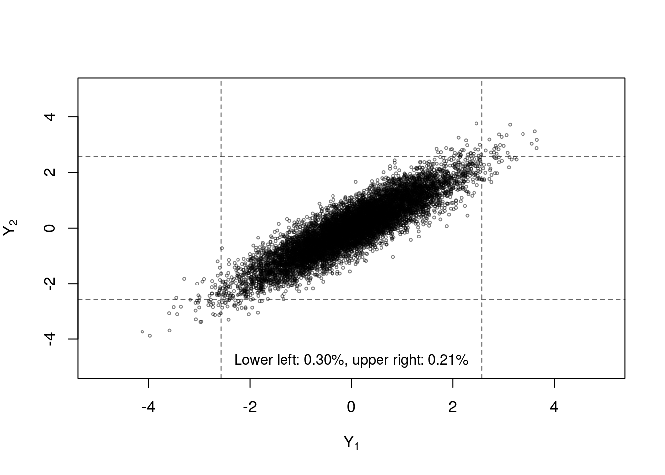

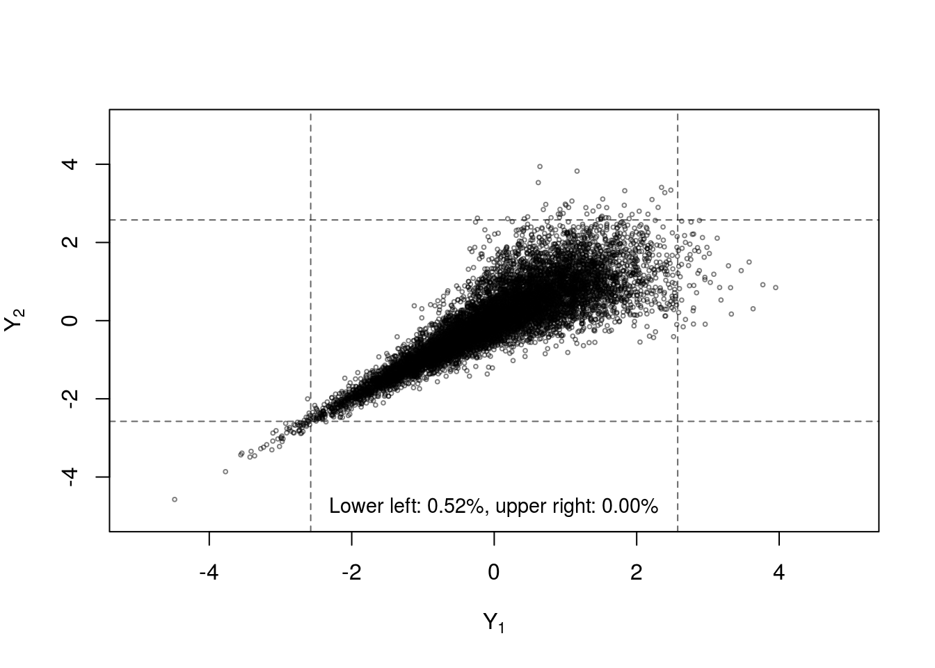
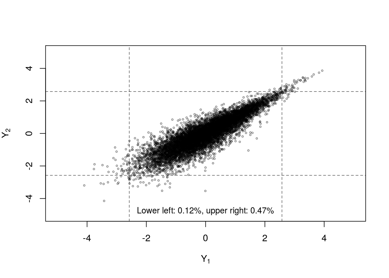
Figure 7: Four samples of n=10000 random draws from bivariate distributions constructed with standard normal margins and Kendall’s \(\tau=0.7\) with (clockwise from top left) normal copula, Student-\(t_3\) copula, Gumbel copula and Clayton copula. Dashed lines indicate the 0.005 and 0.995 quantiles of the standard normal margins.
In practical terms, understanding the various dependence properties of the joint distribution under investigation will help guide the choice of an appropriate copula or copulas to model these properties.
Copula Families
Two of the most popular copula classes are the elliptical copulas, which include multivariate normal and multivariate Student-\(t\) copulas, and the Archimedean copulas. Elliptical distributions have density functions whose contours are concentric ellipses with constant eccentricity. Elliptical copulas are derived by replacing \(H\) and \(F_1^{-1},\ldots,F_d^{-1}\) in equation (2) with the corresponding multivariate df and quantile functions from the elliptical distribution as shown in (4) for the normal distribution. Archimedean copulas can be written in the form \(C(u_1,\ldots,u_d)=\psi^{[-1]}(\psi(u_1) + \cdots + \psi(u_d))\) where \(\psi\) is called the generator function. If the generator function satisfies certain requirements, the formula in the previous sentence will produce a valid copula.
Each of these classes contains many copula families which are specific copula forms indexed by one or more parameters. Table 1 shows common copula families along with desirable properties. A closed-form df is useful for evaluating discrete margins since probabilities are obtained by taking differences in dfs for discrete variables. The desirability of the other properties is related to the dependence structure of the data to be modeled. Nadarajah et al. [23] provides details on over 60 copula families created to represent a large variety of dependence features. Although no family possesses all the desirable properties, there are also several methods for constructing copulas with a combination of characteristics. One method is through mixture copulas, which are weighted sums of other copulas. For example \(C^{mix}(\mathbf{u}|R,\theta_{G},\theta_{C},w_1,w_2)=w_1C_{R}^{Norm}(\mathbf{u}|R) + w_2C^{Gumbel}(\mathbf{u}|\theta_{G}) + w_3C^{Clayton}(\mathbf{u}|\theta_{C})\) where \(w_1,w_2\) and \(w_3=1-w_1-w_2\) are mixture weights. \(C^{mix}\) can accomodate symmetry and both lower and upper tail dependence, but at the price of additional complexity. There are additional techniques for constructing copulas with asymmetrical dependence, non-exhangeable arguments, or copula parameters related to specific quantities of interest such as odds ratios.
| Name | Class | Includes \(M\) and \(\Pi\) | Symmetric | Tail Dependence | Closed-form CDF | Closed-form density |
|---|---|---|---|---|---|---|
| Normal/Gaussian | Elliptical | Yes | Yes | No | No | Yes |
| Student-t | Elliptical | No | Yes | Yes | No | Yes |
| Gumbel | Archimedean | Yes | No | Yes, upper tail | Yes | Yes |
| Clayton | Archimedean | Yes | No | Yes, lower tail | Yes | Yes |
| Frank | Archimedean | Yes | Yes | No | Yes | Yes |
Inference
Equation (1) shows how to construct a multivariate df from univariate dfs and a copula, but in practice neither the margins nor the copula is known. Rather, the investigator collects \(n\) multivariate observations \((y_{i1},\ldots,y_{id}),\; i=1,\ldots,n\) from which the unknown data-generating process is inferred. In clinical trials, the margins are often of primary interest and the general form for each margin is usually assumed to be known while the parameters must be estimated. The inference task is to find a multivariate df that is a good approximation to true data-generating process among the Fréchet class with the given margins. The resulting estimated parameters and multivariate df can be used to assess the effect of intervention on each individual outcome and the dependence between outcomes. This report briefly describes how fully parametric inference is performed for copulas under frequentist and Bayesian paradigms although semiparametric and nonparametric methods for the margins and copula have also been developed [13,22,24–26]. For both paradigms the log-likelihood function is central. In the simplest case of all continuous marginal dfs \(F_1,\ldots,F_d\), differentiation with respect to all \(d\) dimensions can be used to obtain the copula density \(c(u_1,\ldots,u_d)=\frac{\partial^d C(u_1,\ldots,u_d)}{\partial u_1 \cdots \partial u_d}\). Then the multivariate density is \(h(\mathbf{y})=c(F_1(y_1),\ldots,F_d(y_d)) \times \prod_{j=1}^{d} f_j(y_j)\). Assuming the multivariate observations \((y_{i1},\ldots,y_{id})\) are iid, the log-likelihood is: \[\begin{equation} \ell(\mathbf{\gamma}_1,\ldots,\mathbf{\gamma}_d,\mathbf{\theta}) = \sum_{i=1}^{n} \{ \log c_{\theta}(F_1(y_{i1};\mathbf{\gamma}_1),\ldots,F_d(y_{id};\mathbf{\gamma}_d)) + \sum_{j=1}^{d} \log f_j(y_{ij};\mathbf{\gamma}_j) \}\tag{5} \end{equation}\]Likelihood functions for discrete or mixed margins are available in the Technical Supplement.
Frequentist
Maximizing equation (5) with respect to the parameters yields the maximum likelihood estimates, \((\mathbf{\hat{\gamma}}_1,\ldots,\mathbf{\hat{\gamma}}_d,\mathbf{\hat{\theta}})\). The maximization can be performed jointly for the entire likelihood or in a two-stage estimation procedure called inference functions for margins [27]. Inference functions for margins first obtains estimates for all marginal parameters separately and then uses these estimates as fixed values for the margins to estimate the copula parameters. This approach is less statistically efficient than the full maximum likelihood estimator and does not properly account for the variability in the marginal estimates when estimating the copula parameters, but is more computationally efficient if \(d\) is large since it avoids maximization over a high dimensional parameter space.
Bayesian
Bayesian inference provides a principled method of combining prior information concerning parameters with observed data based on Bayes’ Theorem: \[\begin{equation} p(\theta|y)=\frac{p(y|\theta)p(\theta)}{\int p(y|\theta)p(\theta)\,d\theta} \tag{6} \end{equation}\]For copula modeling, \(p(y|\theta)\) in equation (6) is replaced by the likelihood from (5) and \(p(\theta)\) represents prior information (or absence of information) about the marginal and copula parameters. The combination of these two components yields the posterior probability \(p(\theta|y)\) which represents an updated distribution for the parameters conditional on the observed data.
Performing inference for copula models in a Bayesian framework has several advantages. Principal among these is the ability to answer inferential questions using interpretable posterior probabilities as discussed earlier rather than the hypothesis tests and p-values which are dominant in the frequentist paradigm. Bayesian models correctly propagate uncertainty by accounting for the variance in the marginal models when estimating copula parameters [28]. Since the posterior can be iteratively updated as new data are collected, they are also attractive for adaptive or sequential designs [29]. Smith [30,31] describes several circumstances where a Bayesian copula model may be preferred. These include: when the likelihood is difficult to maximize but the posterior can be approximated well using a Monte Carlo approach; when the focus of inference is a dependence measure, quantile, or other statistic for which confidence intervals or p-values are difficult to obtain; when using hierarchical models of copula dependence structure or margins; and when performing penalization for models with a large number of parameters. Finally, by developing appropriate priors Bayesian models can include information from different sources including previous related studies, pre-clinical models, elicited clinical expertise, or observational data sources, although these extensions have not been well explored using copula models.
Copula Regression
In order to use copulas in a clinical trial setting, the basic theory must be extended to include covariates for the groups being compared (dose levels, treatment vs. control, etc.) and possibly other factors.
Regression models for marginal outcomes
The margins can be extended to depend on covariates by replacing each marginal df with a conditional df tied to a regression model. \(F_j(Y_j)\) is replaced by \(F_j(Y_j|X_j)\) where \(X_j\) is a vector of \(p_j\) known covariates for the \(j^{th}\) marginal regression model. In a clinical trial the primary covariate of interest is usually treatment group or dose level and these covariates would be common to all margins, however the \(j\) marginal models are not required to have a common set of covariates or to use the same functional form for covariates. For each \(j=1,\ldots,d\) there is a marginal calibration function \(\varphi_j\) which relates the observed \(X_j\) to the parameters of \(F_j\). One possible marginal calibration function for the location parameter of \(F_j\) is \(\gamma_{j,\mathbf{x}_j}=\varphi_j(\mathbf{x}_j)=E[Y_j|X_j]=\beta_{j0}+\sum_{k=1}^{p_j} \beta_{jk}X_{jk}\). The conditional df based on this calibration function is written \(F_{j}(y_j;\varphi_j(X_j))\).
Regression models for copula parameters
Covariates can also be used to model the copula dependence parameter, using a copula calibration function, \(\theta_{\mathbf{X}}=\zeta(\mathbf{X})\). Including both the marginal and copula calibration functions, the likelihood from equation (5) becomes: \[\begin{equation} \ell(\mathbf{\beta}_1,\ldots,\mathbf{\beta}_d,\mathbf{\theta}) = \sum_{i=1}^{n} \{ \log c_{\theta_{\mathbf{x}}}(F_1(y_{i1}; \varphi_1(x_{i1})), \ldots , F_d(y_{id};\varphi_d(x_{id}))) + \sum_{j=1}^{d} \log f_j(y_{ij};\varphi_j(x_{ij})) \}\tag{7} \end{equation}\]Models where the dependence structure depends on covariates are called conditional copulas and are an active area of research [28,32–34].
Extensions
In addition to the conditional copula models discussed in the previous section, there is extensive literature describing theoretical and methodological extensions related to copula modeling of multivariate survival data [35–41], longitudinal or clustered data [15,42–46], joint longitudinal/survival outcomes [47,48], missing data [49,50] and latent factors underlying the dependence structure [51,52]. Another important area of active research is vine copulas. These models are used to specify multivariate dependence structure with more than 2 dimensions by representing the \(d\)-dimensional copula in terms of \(d \choose 2\) bivariate copulas [13,53–56].
Further details on copulas including technical definitions and proofs, methods for copula construction and sampling, descriptions of available copula families and their properties, inference and diagnostic procedures, and computational algorithms are presented in the texts An Introduction to Copulas by Roger Nelsen [57], Dependence Modeling with Copulas by Harry Joe [13], and Elements of Copula Modeling with R by Hofert et al. [22]. The final text describes the R package copula [58] which was used throughout this report.
References
16. Sklar A. Fonctions de répartition à n dimensions et leurs marges. Publications de l’Institut de Statistique de l’Université de Paris 1959;8:229–31.
17. Genest C, Nešlehová J. A primer on copulas for count data. ASTIN Bulletin [Internet] 2007 [cited 2018 Aug 13];37:475–515. Available from: https://www.cambridge.org/core/product/identifier/S0515036100014963/type/journal_article
18. Denuit M, Lambert P. Constraints on concordance measures in bivariate discrete data. Journal of Multivariate Analysis [Internet] 2005 [cited 2019 Jan 16];93:40–57. Available from: http://linkinghub.elsevier.com/retrieve/pii/S0047259X04000144
19. Niewiadomska-Bugaj M, Kowalczyk T. On grade transformation and its implications for copulas. Brazilian Journal of Probability and Statistics 2005;19:125–37.
20. Rüschendorf L. On the distributional transform, sklar’s theorem, and the empirical copula process. Journal of Statistical Planning and Inference [Internet] 2009 [cited 2019 Jan 16];139:3921–7. Available from: https://linkinghub.elsevier.com/retrieve/pii/S037837580900158X
21. Schweizer B, Wolff EF. On nonparametric measures of dependence for random variables. The Annals of Statistics [Internet] 1981 [cited 2019 Jan 26];9:879–85. Available from: http://projecteuclid.org/euclid.aos/1176345528
22. Hofert M. Elements of copula modeling with r. 1st edition. New York, NY: Springer Berlin Heidelberg; 2018.
23. Nadarajah S, Afuecheta E, Chan S. A compendium of copulas. Statistica [Internet] 2018 [cited 2019 Feb 5];Vol 77:No 4 (2017). Available from: https://rivista-statistica.unibo.it/article/view/7202
13. Joe H. Dependence modeling with copulas. Boca Raton: CRC Press, Taylor & Francis Group; 2015.
24. Hoff P. Extending the rank likelihood for semiparametric copula estimation. The Annals of Applied Statistics [Internet] 2007 [cited 2018 Oct 12];1:265–83. Available from: http://projecteuclid.org/euclid.aoas/1183143739
26. Ning S, Shephard N. A nonparametric bayesian approach to copula estimation. arXiv:1702.07089 [stat] [Internet] 2017 [cited 2018 Sep 6];Available from: http://arxiv.org/abs/1702.07089
27. Joe H, Xu JJ. The estimation method of inference functions for margins for multivariate models. The University of British Columbia [Internet] 1996 [cited 2019 Feb 6];Available from: https://doi.library.ubc.ca/10.14288/1.0225985
28. Craiu VR, Sabeti A. In mixed company: Bayesian inference for bivariate conditional copula models with discrete and continuous outcomes. Journal of Multivariate Analysis [Internet] 2012 [cited 2018 Sep 27];110:106–20. Available from: http://linkinghub.elsevier.com/retrieve/pii/S0047259X12000796
29. Yuan Y, Yin G. Bayesian phase i/II adaptively randomized oncology trials with combined drugs. The Annals of Applied Statistics [Internet] 2011 [cited 2018 Jul 26];5:924–42. Available from: http://arxiv.org/abs/1108.1614
30. Smith MS, Khaled MA. Estimation of copula models with discrete margins via bayesian data augmentation. Journal of the American Statistical Association [Internet] 2012 [cited 2018 Oct 12];107:290–303. Available from: http://www.tandfonline.com/doi/abs/10.1080/01621459.2011.644501
31. Smith MS. Bayesian approaches to copula modelling [Internet]. In: Damien P, Dellaportas P, Polson NG, Stephens DA, editors. Bayesian theory and applications. Oxford University Press; 2013 [cited 2019 Jan 25]. pages 336–58.Available from: http://www.oxfordscholarship.com/view/10.1093/acprof:oso/9780199695607.001.0001/acprof-9780199695607-chapter-17
32. Acar EF, Craiu RV, Yao F. Statistical testing of covariate effects in conditional copula models. Electronic Journal of Statistics [Internet] 2013 [cited 2018 Sep 27];7:2822–50. Available from: http://projecteuclid.org/euclid.ejs/1385995292
34. Fermanian J-D, Lopez O. Single-index copulas. Journal of Multivariate Analysis [Internet] 2018 [cited 2018 Sep 27];165:27–55. Available from: https://linkinghub.elsevier.com/retrieve/pii/S0047259X17303032
35. Shih JH, Louis TA. Inferences on the association parameter in copula models for bivariate survival data. Biometrics [Internet] 1995 [cited 2018 Oct 23];51:1384–99. Available from: https://www.jstor.org/stable/2533269?origin=crossref
41. Weber EM, Titman AC. Quantifying the association between progression-free survival and overall survival in oncology trials using kendall’s tau: Correlation between progression-free survival and overall survival. Statistics in Medicine [Internet] 2018 [cited 2018 Oct 17];Available from: http://doi.wiley.com/10.1002/sim.8001
15. Meester SG, MacKay J. A parametric model for cluster correlated categorical data. Biometrics [Internet] 1994 [cited 2019 Jan 26];50:954–63. Available from: https://www.jstor.org/stable/2533435?origin=crossref
42. Eluru N, Paleti R, Pendyala RM, Bhat CR. Modeling injury severity of multiple occupants of vehicles: Copula-based multivariate approach. Transportation Research Record: Journal of the Transportation Research Board [Internet] 2010 [cited 2019 Jan 27];2165:1–11. Available from: http://journals.sagepub.com/doi/10.3141/2165-01
46. Kwak M. Estimation and inference on the joint conditional distribution for bivariate longitudinal data using gaussian copula. Journal of the Korean Statistical Society [Internet] 2017 [cited 2019 Jan 4];46:349–64. Available from: https://linkinghub.elsevier.com/retrieve/pii/S1226319216300606
47. Ganjali M, Baghfalaki T. A copula approach to joint modeling of longitudinal measurements and survival times using monte carlo expectation-maximization with application to AIDS studies. Journal of Biopharmaceutical Statistics [Internet] 2015 [cited 2018 Oct 12];25:1077–99. Available from: http://www.tandfonline.com/doi/full/10.1080/10543406.2014.971584
48. Kürüm E, Jeske DR, Behrendt CE, Lee P. A copula model for joint modeling of longitudinal and time-invariant mixed outcomes: Joint modeling of longitudinal and time-invariant mixed outcomes. Statistics in Medicine [Internet] 2018 [cited 2018 Jul 9];1–13. Available from: http://doi.wiley.com/10.1002/sim.7855
49. Ding W. Copula regression models for the analysis of correlated data with missing values. 2015;
50. Gomes M, Radice R, Camarena Brenes J, Marra G. Copula selection models for non-gaussian outcomes that are missing not at random: Copula selection models for non-normal data. Statistics in Medicine [Internet] 2019 [cited 2019 Jan 6];38:480–96. Available from: http://doi.wiley.com/10.1002/sim.7988
51. Krupskii P, Joe H. Factor copula models for multivariate data. Journal of Multivariate Analysis [Internet] 2013 [cited 2019 Jan 15];120:85–101. Available from: https://linkinghub.elsevier.com/retrieve/pii/S0047259X13000870
52. Tan BK, Panagiotelis A, Athanasopoulos G. Bayesian inference for the one-factor copula model. Journal of Computational and Graphical Statistics [Internet] 2018 [cited 2018 Sep 18];1–19. Available from: https://www.tandfonline.com/doi/full/10.1080/10618600.2018.1482765
53. Smith M, Min A, Almeida C, Czado C. Modeling longitudinal data using a pair-copula decomposition of serial dependence. Journal of the American Statistical Association [Internet] 2010 [cited 2018 Oct 12];105:1467–79. Available from: http://www.tandfonline.com/doi/abs/10.1198/jasa.2010.tm09572
56. Barthel N, Geerdens C, Czado C, Janssen P. Dependence modeling for recurrent event times subject to right‐censoring with d‐vine copulas. Biometrics [Internet] 2018 [cited 2018 Dec 17];Available from: https://onlinelibrary.wiley.com/doi/abs/10.1111/biom.13014
57. Nelsen RB. An introduction to copulas. 2nd ed. New York: Springer; 2006.
58. Hofert M, Kojadinovic I, Maechler M, Yan J. Copula: Multivariate dependence with copulas [Internet]. 2016. Available from: http://cran.r-project.org/package=copula