Applications
Benefit-Risk Analysis
Costa and Drury [14] present a simulation involving mixed bivariate outcomes to demonstrate the use of joint copula models for benefit-risk analysis. The simulation assumes a two-arm parallel design with total sample size of n=200 and 1:1 randomization to either treatment \(t=1\) (placebo) or \(t=2\) (active drug). The bivariate response for individual \(i\) is \(y_i=(y_{i1},y_{i2})\) where \(y_{i1}\) is the efficacy outcome assumed to be normal with mean \(\mu_{t}\) and variance \(\sigma_{t}^2\) and \(y_{i2}\) is a binary indicator of whether the participant experienced an adverse event (AE) which follows a Bernoulli distribution with probability \(p_{t}\). A vector of indicators \(x_i=(x_{i1},x_{i2})\) specifies treatment in either the placebo or active arm. Probit regression – which assumes a latent normal distribution underlying the binary observations – was used for the marginal safety outcome while an OLS model was used for efficacy. A normal conditional copula that allows different dependence in each treatment group was used to connect the two marginal models. The overall model specification is: \[\begin{gather*} y_{i1} \sim Normal(\mu_{t},\sigma_{t}), \,\, \mu_{t} = x_{i1}\beta_{11} + x_{i2}\beta_{12}, \,\, \sigma_{t} = x_{i1}s_1 + x_{i2}s_2\\ y_{i2} \sim Bernoulli(p_{t}), \,\, \Phi^{-1}(p_i) = x_{i1}\beta_{21} + x_{i2}\beta_{22}\\ H_{\theta_{t}}(y_{i1},y_{i2})=C_{\theta_{t}}^{Norm}(F_1(y_{i1}|\mu_{t},\sigma_{t}),F_2(y_{i2}|p_{t})), \,\, \theta_{t} = x_{i1}\omega_{1} + x_{i2} \omega_{2} \end{gather*}\]where the \(\beta_{jt}\) are effect parameters, \(s_t\) are dispersion parameters, and \(\omega_t\) are copula dependency parameters for treatment \(t\). The copula dependence parameter, \(\theta_t\), is the poly-serial correlation which measures the correlation between the normal efficacy outcome and the latent normal distribution assumed to underlie the binary safety outcome. The Pearson correlation between the outcomes is \(\rho_t=\theta_t\phi[\Phi^{-1}(p_t)]/\sqrt{p_t(1-p_t)}\) where \(\phi\) is the standard normal density. Note that the correlation is a function of both \(\theta_t\) and the marginal \(p_t\) parameter.
The values used for the simulation are representative of data from a real respiratory clinical trial. For the placebo group \(\mu_1 = -150\), \(\sigma_1^2=100^2\), \(p_1=0.1\) and \(\rho_1=0.1\) and for the treatment group \(\mu_2 = -50\), \(\sigma_2^2=100^2\), \(p_2=0.4\) and \(\rho_2=0.6\). The efficacy, AE rate, and correlation between them are different by intervention group with weak dependence for placebo and moderate dependence for active drug.
## Benefit-Risk application

# Simulate data
set.seed(4283)

# function to get copula parameter given rho and p; see Costa section 3.1.2
getTheta <- function(rho,p){  (rho*sqrt(p*(1-p))) / dnorm(qnorm(p)) }

# number of samples per arm
n<-100

# placebo group
mu_1 <- -150
sigma2_1 <- 100^2
p_1 <- 0.1
rho_1 <- 0.1

# normal copula
nc_p<-normalCopula( getTheta(rho=rho_1, p=p_1)  )

pbo_dist <- mvdc(nc_p, margins = c("norm","binom"),
                paramMargins = list(list(mean = mu_1, sd = sqrt(sigma2_1)),
                                    list(size = 1, prob = p_1)) )

pbo_samps<-rMvdc(n, pbo_dist)

if (0){ # check simulated values
mean(pbo_samps[,1]) # mu_1
sd(pbo_samps[,1]) # sigma_1
mean(pbo_samps[,2]) #p_1
cor(pbo_samps[,1],pbo_samps[,2]) # rho_1 (Pearson corr)
}

# treatment
mu_2 <- -50
sigma2_2 <- 100^2
p_2 <- 0.4
rho_2 <- 0.6

# normal copula
nc_t<-normalCopula( getTheta(rho=rho_2, p=p_2)  )

trt_dist <- mvdc(nc_t, margins = c("norm","binom"),
                paramMargins = list(list(mean = mu_2, sd = sqrt(sigma2_2)),
                                    list(size = 1, prob = p_2)) )

trt_samps<-rMvdc(n, trt_dist)

if (0){ # check simulated values
mean(trt_samps[,1]) # mu_2
sd(trt_samps[,1]) # sigma_2
mean(trt_samps[,2]) #p_2
cor(trt_samps[,1],trt_samps[,2]) # rho_2 (Pearson corr)
}

#combine placebo and treatment data
dat <- rbind(pbo_samps,trt_samps) %>% cbind(sort(rep(c(0,1),n)),
                                            sort(rep(c(0,1),n),decreasing=TRUE),
                                            sort(rep(c(0,1),n))) %>% as.data.frame()
names(dat) <- c("efficacy","safety","treatment","trt1","trt2")

dat_lab <- dat
dat_lab %<>% mutate(treatment=factor(treatment, labels=c("placebo","active")),
                   safety=factor(safety, labels=c("no AE","AE")))
The histograms of efficacy by treatment and AE status for the simulated data in Figure 8 confirm that the highest efficacy was observed for those in the active treatment group with an adverse event.
ggplot(dat_lab, aes(x=efficacy, fill=treatment)) +
  geom_histogram(bins=20, alpha=0.75) + facet_grid(treatment~safety)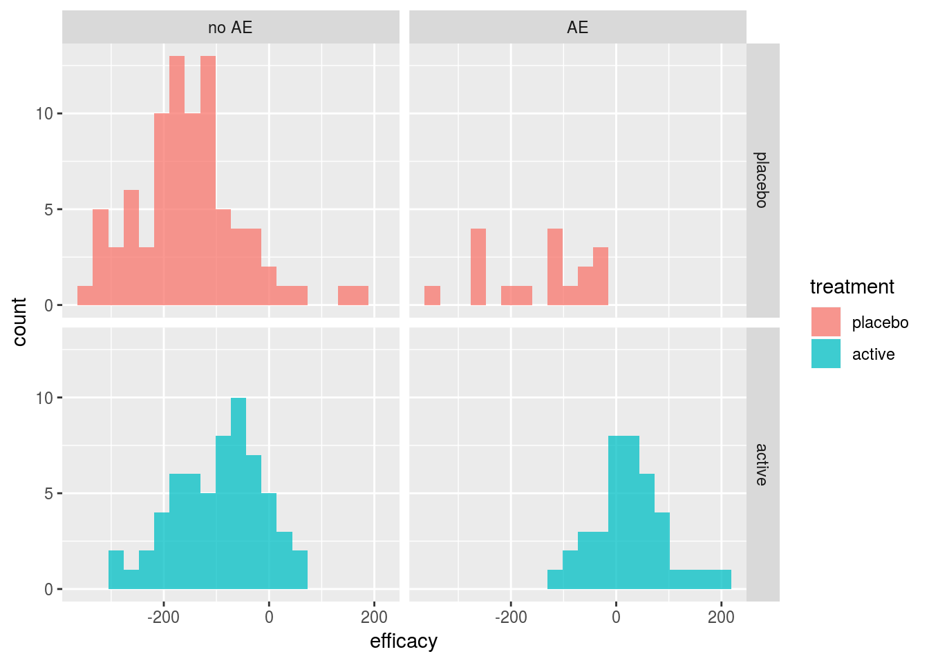
Figure 8: Simulated data from Costa and Drury Benefit-Risk Example
Weakly informative normal priors were used for \(\beta\) parameters and an inverse gamma with shape and scale parameters both equal to 0.001 was used for \(\sigma\). For the copula parameter \(\theta\), a flat uniform distribution on the interval [-1,1] was used. To explore the effect of fitting the joint copula model, each marginal model was also fit separately assuming independence between the outcomes. The R package rstan [59] was used to draw samples from the posterior distribution using the default No-U-Turn-Sampler (NUTS) MCMC algorithm, an implementation of Hamiltonian Monte Carlo. For each model, 4 chains with 1000 warmup iterations and 2000 sampling iterations were used resulting in 8000 samples from each posterior distribution. Diagnostics for the MCMC samples are shown in the Technical Supplement.
## Stan code for B-R model
# http://mc-stan.org/rstan/
rstan_options(auto_write = TRUE)

# marginal models assuming independence
mod0a_code <- "
data {
  int N;
  matrix[N, 2] x;
  vector[N] y1;
}
parameters {
  // params for continuous (efficacy) outcome
   vector[2] beta1;
   real<lower=0> sigma;
}
model {
  vector[N] mu;

  // priors
  beta1 ~ normal(0,1000);
  sigma ~ inv_gamma(0.001,0.001);

  // marginal for continuous (efficacy) outcome
  mu = beta1[1]*x[,1] + beta1[2]*x[,2];
  y1 ~ normal(mu, sigma);
}
"

mod0b_code <- "
data {
  int N;
  matrix[N, 2] x;
  int<lower=0, upper=1> y2[N];
}
parameters {
  //params for binary (safety) outcome
   vector[2] beta2;
}
model {
  vector[N] p;

  // priors
  beta2 ~ normal(0,1000);

  // marginal for binary (safety) outcome
  p = beta2[1]*x[,1] + beta2[2]*x[,2];
  y2 ~ bernoulli(Phi(p));
  }
generated quantities {
  vector[2] p;

  p[1] = Phi(beta2[1]);
  p[2] = Phi(beta2[2]);
}
"

# joint model
mod_code <- "
data {
  int N;
  matrix[N, 2] x;
  vector[N] y1;
  int<lower=0, upper=1> y2[N];
}
parameters {
  // params for continuous (efficacy) outcome
  vector[2] beta1;
  vector<lower=0>[2] s;

  //params for binary (safety) outcome
  vector[2] beta2;

  // copula dependence param
  vector<lower=-1, upper=1>[2] omega;
}
model {
  vector[N] mu;
  vector[N] sigma;
  vector[N] p;
  vector[N] theta;

  // priors
  beta1 ~ normal(0,1000);
  beta2 ~ normal(0,1000);
  s ~ inv_gamma(0.001,0.001);

  // marginal for continuous (efficacy) outcome
  mu = beta1[1]*x[,1] + beta1[2]*x[,2];
  sigma = s[1]*x[,1] + s[2]*x[,2];

  // marginal for binary (safety) outcome
  p = Phi(beta2[1]*x[,1] + beta2[2]*x[,2]);

  // copula dependence parameter
  theta = omega[1]*x[,1]+omega[2]*x[,2];

  // build log-likelihood
  for(i in 1:N){
    target += normal_lpdf(y1[i]|mu[i],sigma[i]);
      if (y2[i]==0) {
        target += normal_lcdf((inv_Phi(1-p[i])-theta[i]*
inv_Phi(normal_cdf(y1[i],mu[i],sigma[i])))/sqrt(1-theta[i]^2)|0,1);
      } else {
        target += normal_lccdf((inv_Phi(1-p[i])-theta[i]*
inv_Phi(normal_cdf(y1[i],mu[i],sigma[i])))/sqrt(1-theta[i]^2)|0,1);
      }
    }

}
generated quantities {
  vector[2] mu;
  vector[2] p;
  vector[2] theta;
  vector[2] rho;

  mu[1] = beta1[1];
  mu[2] = beta1[2];

  p[1] = Phi(beta2[1]);
  p[2] = Phi(beta2[2]);

  theta[1] = omega[1];
  theta[2] = omega[2];

  rho[1] = theta[1]*exp(normal_lpdf(inv_Phi(p[1])|0,1))/sqrt(p[1]*(1-p[1]));
  rho[2] = theta[2]*exp(normal_lpdf(inv_Phi(p[2])|0,1))/sqrt(p[2]*(1-p[2]));
}
"
Table 2 summarizes the mean, Monte Carlo standard error, standard deviation, and quantiles of the posterior distributions for parameters \(\mu_t\), \(p_t\), \(\rho_t\), and \(\theta_t\) from the normal copula model. The number of effective samples – a function of the correlation between sample draws – along with Rhat – a measure of MCMC convergence – are also shown. The model performs reasonable well with posterior median estimates close to the true values for all parameters except the correlation between outcomes \(\rho_1\) and adverse event rate \(p_1\) in the placebo group.
br_tab <- round(summary(br_fit, pars=c("mu","p","rho","theta"))$summary,2) | Mean | MCSE Mean | SD | 2.5% | 25% | 50% | 75% | 97.5% | eff. num. samps | Rhat | |
|---|---|---|---|---|---|---|---|---|---|---|
| \(\mu_1\) | -152.97 | 0.11 | 10.17 | -172.84 | -159.84 | -153.08 | -146.05 | -133.05 | 8000.00 | 1 |
| \(\mu_2\) | -49.60 | 0.13 | 9.88 | -68.88 | -56.19 | -49.58 | -42.92 | -30.33 | 5976.45 | 1 |
| \(p_1\) | 0.17 | 0.00 | 0.04 | 0.11 | 0.15 | 0.17 | 0.20 | 0.25 | 8000.00 | 1 |
| \(p_2\) | 0.38 | 0.00 | 0.05 | 0.29 | 0.35 | 0.38 | 0.41 | 0.48 | 5486.21 | 1 |
| \(\rho_1\) | 0.01 | 0.00 | 0.09 | -0.17 | -0.05 | 0.01 | 0.08 | 0.19 | 8000.00 | 1 |
| \(\rho_2\) | 0.61 | 0.00 | 0.05 | 0.49 | 0.58 | 0.61 | 0.64 | 0.69 | 7065.79 | 1 |
| \(\theta_1\) | 0.02 | 0.00 | 0.14 | -0.26 | -0.08 | 0.02 | 0.11 | 0.29 | 8000.00 | 1 |
| \(\theta_2\) | 0.77 | 0.00 | 0.06 | 0.63 | 0.74 | 0.78 | 0.82 | 0.88 | 7167.84 | 1 |
Using the posterior samples, the difference in mean efficacy response \(\mu_2-\mu_1\) and the difference in probability of adverse events \(p_2 - p_1\) was calculated for the normal copula and independence models. Figures 9 and 10 plot the results along with overlaid density curves and marginal histograms. The marginal histograms are nearly identical for both models, but the efficacy and safety treatment differences from the copula model have a clear positive dependence while there is no relationship between them in the independence model as expected.
#calculate treatment effect (efficacy) and risk difference (safety)
posterior_mu <- extract(br_fit, pars=c("mu[1]","mu[2]"))
mu <- do.call(cbind.data.frame, posterior_mu) %>% mutate(mu_diff=`mu[2]`-`mu[1]`)

posterior_p <- extract(br_fit, pars=c("p[1]","p[2]"))
p <- do.call(cbind.data.frame, posterior_p) %>% mutate(p_diff=`p[2]`-`p[1]`)

diffs<-cbind(mu,p)

# assuming independence model
posterior_mu0 <- extract(fit0a, pars=c("beta1[1]","beta1[2]"))
mu0 <- do.call(cbind.data.frame, posterior_mu0) %>% mutate(mu_diff=`beta1[2]`-`beta1[1]`)

posterior_p0 <- extract(fit0b, pars=c("p[1]","p[2]"))
p0 <- do.call(cbind.data.frame, posterior_p0) %>% mutate(p_diff=`p[2]`-`p[1]`)

diffs0<-cbind(mu0,p0)

save(br_fit, br_tab, diffs, diffs0, file="br_mod_out.RData")
# scatterplot with histogram margins
mu_diff_hist <- plot_ly(x=diffs$mu_diff, type="histogram", nbinsx = 25,
color=I("steelblue"), showlegend=FALSE)
p_diff_hist <- plot_ly(y=diffs$p_diff,type="histogram", nbinsy = 25,
color=I("steelblue"),showlegend=FALSE)
scatterplt <- plot_ly(x=diffs$mu_diff,y=diffs$p_diff) %>%
add_histogram2dcontour(showscale=FALSE, ncontours=10, contours = list(coloring='none'),
color=I("steelblue"), line=list(width=2,smoothing=1.1),
showlegend=FALSE) %>%
add_markers(x = diffs$mu_diff, y = diffs$p_diff, color=I("black"),
marker=list(size=3), alpha=.25,showlegend=FALSE) %>%
layout(xaxis=list(title ="Treatment Difference (Efficacy)"),
yaxis=list(title = "Treatment Difference (Safety)"))
plt_emp <- plotly_empty(type="scatter",mode="markers")
marg_plot<-subplot(mu_diff_hist, plt_emp, scatterplt, p_diff_hist,
nrows = 2, heights = c(.2, .8), widths = c(.8,.2),
shareX=TRUE, shareY=TRUE)
marg_plotFigure 9: Posterior treatment effect vs. safety risk difference posterior estimates from normal copula model
# scatterplot with histogram margins
mu_diff_hist0 <- plot_ly(x=diffs0$mu_diff, type="histogram", nbinsx = 25,
                        color=I("steelblue"), showlegend=FALSE)

p_diff_hist0 <- plot_ly(y=diffs0$p_diff, type="histogram", nbinsy = 25,
                       color=I("steelblue"),showlegend=FALSE)

scatterplt0 <- plot_ly(x=diffs0$mu_diff, y=diffs0$p_diff) %>%
    add_histogram2dcontour(showscale=FALSE, ncontours=10, contours = list(coloring='none'),
                           color=I("steelblue"), line=list(width=2,smoothing=1.1),
                           showlegend=FALSE) %>%
    add_markers(x = diffs0$mu_diff, y = diffs0$p_diff, color=I("black"),
                marker=list(size=3), alpha=.25,showlegend=FALSE) %>%
    layout(xaxis=list(title ="Treatment Difference (Efficacy)"),
           yaxis=list(title = "Treatment Difference (Safety)"))

marg_plot0 <- subplot(mu_diff_hist0, plt_emp, scatterplt0, p_diff_hist0,
 nrows = 2, heights = c(.2, .8), widths = c(.8,.2),
 shareX=TRUE, shareY=TRUE)

marg_plot0
Figure 10: Posterior treatment effect vs. safety risk difference posterior estimates from independence model
One event of interest involving both outcomes is the probability of technical success (POTS). The POTS is the probability that the difference in efficacy is greater than or equal to threshold \(\Delta_E\) and the difference in AE risk is less than or equal to threshold \(\Delta_S\). Figure 11 shows the POTS across a range of efficacy and safety values. There is a very low posterior probability that the active drug simultaneously increases efficacy over 110 and has risk difference less than 0.1 (bottom right of plot). Similarly, the probability that the drug improves efficacy by at least 70 and increases risk by 0.5 or less compared to placebo is near \(100\%\) (top left corner of plot). All the pairs of efficacy and safety thresholds along a contour have the same POTS and can be used to quantify the risk-benefit tradeoff.
Costa and Drury achieved similar results using a generalized linear mixed model (GLMM), but note that the copula approach has several advantages including direct interpretation of the marginal model parameters as population-level estimates (compared to subject level estimates in GLMM) and the flexibility to easily model different dependence structures.
# probability of technical success
potus<- function(delta_e, delta_p, dat=diffs){

  potus0 <- function(delta_e, delta_p, dat){
    mean(dat$mu_diff>=delta_e & dat$p_diff<=delta_p)*100
  }

  #vectorize
  mapply(function(x,y) potus0(x,y,dat), delta_e, delta_p)
}

de<-seq(70,130,length=50)
ds<-seq(0,0.5,length=50)
pp<-outer(de,ds,potus)
pp0<-outer(de,ds,potus,dat=diffs0)

# color scheme
num_cols<-20
potus_col <- rev(rainbow(20, start = 0/6, end = 4/6))plot_ly(x=de, y=ds, z=t(pp), type = "contour", colors=potus_col,
contours = list(coloring = 'heatmap', showlabels = TRUE) ) %>%
layout(xaxis=list(title ="Δ<sub>E</sub>"), yaxis=list(title = "Δ<sub>S</sub>"))Figure 11: Benefit-Risk contour plot for probability of technical success \(Pr(\mu_2-\mu_1 \ge \Delta_E \text{ and }p_2-p_1 \le \Delta_S)\) from normal copula model
Clustered Data
Meester and MacKay [15] present a different use of copulas. In this case, there is a single outcome of interest – whether or not OME was cured – and the copula is used to account for dependence between ears for an individual. The study randomized 62 children with unilateral OME and 44 children with bilateral OME to the cefaclor arm. In addition, 66 children with unilateral OME and 31 children with bilateral OME were randomized to the amoxicillin arm. Age was given in categories of \(<2\) yr, \(2-5\) yr, and \(\ge\) 6 yr. A binary indicator of cure (yes/no) was recorded for each affected ear after 14 days of treatment.
The logistic regression model for each ear is: \(\text{logit}[Pr(\text{ear cured}_i|\mathbf{X}_i=\mathbf{x}_i)]=\beta_0 + \beta_1x_{\text{amox},i} + \beta_2 x_{\text{age } 2-5,i} + \beta_3 x_{\text{age}\ge 6,i}=\mathbf{\beta'x_i}\) or equivalently \(p_i = Pr(\text{ear cured}_i|\mathbf{x}_i)=\frac{1}{1+\exp(-\mathbf{\beta'x_i})}\). For the 128 children with unilateral OME, this completes the model specification. For the 75 children with bilateral OME, the dependence between the left and right ear was modeled using the same logistic regression for each margin and a Frank copula with the form \(C_{\alpha}^{Frank}(u_1,u_2)=-\frac{1}{\alpha}\log\left(1+\frac{(\exp(-\alpha u_1)-1)(\exp(-\alpha u_2)-1)}{\exp(-\alpha)-1} \right),\) \((u_1,u_2) \in [0,1]^2,\, \alpha \in \mathbb{R}\ \backslash \{0\}\) to specify the joint distribution using equation (1) in Sklar’s theorem. The values \(u_1\) and \(u_2\) are pseudo-observations calculated using \(F_{Y_i}(y_i)=u_i\) where \(F_{Y_i}\) is the univariate Bernoulli df with parameter \(p_i\) calculated from the logistic model. For the Frank copula, positive dependence increases as \(\alpha \to \infty\) and negative dependence increases as \(\alpha \to -\infty\); \(\alpha=0\) represents independence. The complete log-likelihood is specified by adding the logistic regression model log-likelhoods from those with univariate data to the copula log-likelihoods from those with bivariate data. Because the copula marginal models and the individual logistic regression model are the same, the parameters of interest can be estimated consistently.
## OME data
load("OME_dat.RData")

# make bilateral data wide
bi_dat_wide <- reshape(bi_dat,v.names="cured",direction="wide",
                       idvar="id", timevar="ear")

ome_dat<-rbind(uni_dat,bi_dat)
ome_dat<-ome_dat[,c('id','entry','age','trt','cured')]

# design matrices for unilateral and bilateral data
Xmat1 <- model.matrix(~age+trt, data=uni_dat)
Xmat2 <- model.matrix(~age+trt, data=bi_dat_wide)
## functions for OME application based on code from Hofert et al.
##' @title Marginal conditional negative log-likelihood
##' @param beta.m parameter vector defining the marginal calibration map
##' @param y vector of values of one of the three scores
##' @param x design matrix
##' @param pobs logical indicating whether, additionally, the parametric
##' pseudo-observations shall be computed and returned
##' @return -log-likelihood and, possibly, the parametric pseudo-observations
nmLL <- function(beta.m, y, x, pobs = FALSE) {
np <- ncol(x) # number of parameters
eta_i <- x %*% beta.m[1:np]
p_i <- plogis(eta_i)
nLL <- -sum(y*log(p_i) + (1-y)*log(1-p_i))
if (!pobs) nLL else
list(nLL = nLL, U = pbinom(y, size=1, prob=p_i),
U_prime = pbinom(y-1, size=1, prob=p_i))
}
##' @title Full conditional negative log-likelihood function
##' @param par param. vector defining the marg. and copula calibration maps
##' @param copula a bivariate one-parameter copula object
##' @return -log-likelihood
nfLL <- function(par, copula)
{
beta <- par[1] # copula parameter
tc <- tryCatch(copula <- setTheta(copula, beta), # try to set parameters
error = function(e) NULL)
if (is.null(tc)) return(-Inf) # in case of failure, return -Inf
beta.m <- par[2:5] #marginal model parameters
#unilateral data log-likelihood
nmLL.1 <- nmLL(beta.m, uni_dat[,"cured"], Xmat1)
## Marginal log-likelihood eval for bilateral data and computing the
## corresponding parametric pseudo-observations
nmLL.2 <- nmLL(beta.m, bi_dat_wide[,"cured.1"], Xmat2, pobs = TRUE)
nmLL.3 <- nmLL(beta.m, bi_dat_wide[,"cured.2"], Xmat2, pobs = TRUE)
## In case of invalid evaluation of the likelihoods, return -Inf
if (any(is.na(c(nmLL.1, nmLL.2$nLL, nmLL.3$nLL)))) return(-Inf)
## Parametric pseudo-observations
U2<-nmLL.2$U
U2_prime<-nmLL.2$U_prime
U3<-nmLL.3$U
U3_prime<-nmLL.3$U_prime
## -log-likelihood for joint dist. using differences
cP <- pCopula(cbind(U2,U3), copula=copula) -
pCopula(cbind(U2_prime,U3), copula=copula) -
pCopula(cbind(U2,U3_prime), copula=copula) +
pCopula(cbind(U2_prime,U3_prime), copula=copula)
cl <- -sum( log(cP) )
# complete -log-likelihood with unilateral and bilateral data contributions
cl + nmLL.1
}
# initialize marginal parameters at glm est. assuming independence
fit_init<-glm(cured~age+trt, dat=ome_dat, family="binomial")
# initialize copula parameter by estimating unadjusted spearman's rho
rho <- cor(bi_dat_wide$cured.1, bi_dat_wide$cured.2, method = "spearman")
# function to get alpha estimate for initialization
alp_fun <-function(alpha, r) {
(1-alpha*exp(-alpha/2)-exp(-alpha))*(exp(-alpha/2)-1)^(-2) - r
}
alp_init <- uniroot(alp_fun,c(-10,10), tol = 0.0001, r=rho)$root
init_vals <- c(alp_init, coef(fit_init)[1:4])
# get MLE for copula model using optim
cl_fit<-optim(init_vals, nfLL, copula=frankCopula(dim=2),
method = "Nelder-Mead", hessian=TRUE)
cov_cl_fit <- solve(cl_fit$hessian)
se_cl_fit <- sqrt(diag(cov_cl_fit))
# compare to fit under independence assumption
cl_fit2<-optim(c(0,init_vals[2:5]), nfLL, copula=indepCopula(dim=2),
method = "Nelder-Mead", hessian=TRUE)
cov_cl_fit2 <- solve(cl_fit2$hessian[2:5,2:5])
se_cl_fit2 <- sqrt(diag(cov_cl_fit2))
if (0){
round(2*5+2*cl_fit[['value']],2) # Frank copula model AIC = 2p - 2 log-likelihood
round(2*4+2*cl_fit2[['value']],2) # Ind model AIC = 2p - 2 log-likelihood
alp_fun(cl_fit[['par']][[1]],0) # est of spearman's rho
}The maximum likelihood estimates and standard errors were calculated using the optim function with the default ‘Nelder-Mead’ algorithm to minimize the negative log-likelihood. Table 3 shows parameter estimates, standard errors and odds ratios for the regression parameters.
The copula parameter estimate is 8.294 (equivalent to Spearman’s \(\rho=\) 0.897) which represents strong dependence within individuals. The regression coefficients show that both age and treatment have a significant effect. Older children have significantly higher odds of cure compared to those \(<2\) yr after adjusting for treatment group (OR and \(95\%\) confidence intervals; age 2-5 yr \(_{2.24}5.007_{11.21}\); age \(\ge\) 6 yr \(_{1.65}3.21_{6.25}\)). Those treated with amoxicillin had a significantly lower odds of cure compared to cefaclor (OR and \(95\%\) confidence interval; \(_{0.26}0.454_{0.80}\)).
Meester and MacKay produce similar results using a GEE model for the correlation within individuals, but note that because GEE is a quasi-likelihood method, it cannot be used if a full likelihood is required. For example, different parametric copula models can be compared using AIC. In this example, the AIC for the fitted Frank copula model is 331.92 while a model using an independence copula (which has no copula parameter to estimate) has AIC of 361.09 indicating that the Frank model provides a better fit.
cl_est <- cl_fit$par

cl_tab <- data.frame(Est=round(cl_est,3), SE=round(se_cl_fit,3), OR = c("", paste0(
       round(exp(cl_est[2:5]),3), " (",
       round(exp(cl_est[2:5]+qnorm(0.025)*se_cl_fit[2:5]),2),", ",
       round(exp(cl_est[2:5]-qnorm(0.025)*se_cl_fit[2:5]),2), ")"))
  )

rownames(cl_tab)<-c("$\\alpha$","(intercept)","Age $\\ge$ 6 yr (ref. $<$2 yr)","Age 2-5 yr (ref. $<$2 yr)","Amoxicillin (ref. Cefaclor)")| Estimate | SE Estimate | OR (95% CI) | |
|---|---|---|---|
| \(\alpha\) | 8.294 | 2.568 | |
| (intercept) | -0.474 | 0.293 | 0.623 (0.35, 1.11) |
| Age \(\ge\) 6 yr (ref. $<$2 yr) | 1.166 | 0.340 | 3.21 (1.65, 6.25) |
| Age 2-5 yr (ref. $<$2 yr) | 1.611 | 0.411 | 5.007 (2.24, 11.21) |
| Amoxicillin (ref. Cefaclor) | -0.790 | 0.289 | 0.454 (0.26, 0.8) |
This report has described only two applications of copula modeling, but there are several additional settings where these models are used in the context of clinical trials. In addition to survival and longitudinal outcomes, one of the most common applications of copula modeling is in early phase dose-finding trials where the jointly estimated toxicity and efficacy curves are combined with clinical decision rules for maximum tolerable dose and minimal effective dose to find the optimal dose for future studies. Several designs have been proposed and evaluated [60–63] and there has also been work on optimal design for copula models [64–66]. Copulas have also been used to assess the joint distribution between surrogate and true outcomes [67,68].
References
14. Costa MJ, Drury T. Bayesian joint modelling of benefit and risk in drug development. Pharmaceutical Statistics [Internet] 2018 [cited 2018 Mar 15];Available from: http://doi.wiley.com/10.1002/pst.1852
59. Stan Development Team. RStan: The r interface to stan [Internet]. 2018. Available from: http://mc-stan.org/
15. Meester SG, MacKay J. A parametric model for cluster correlated categorical data. Biometrics [Internet] 1994 [cited 2019 Jan 26];50:954–63. Available from: https://www.jstor.org/stable/2533435?origin=crossref
60. Thall PF, Cook JD. Dose-finding based on efficacy-toxicity trade-offs. Biometrics [Internet] 2004 [cited 2018 Oct 23];60:684–93. Available from: http://doi.wiley.com/10.1111/j.0006-341X.2004.00218.x
63. Cunanan K, Koopmeiners JS. Evaluating the performance of copula models in phase i-II clinical trials under model misspecification. BMC Medical Research Methodology [Internet] 2014 [cited 2018 Jul 26];14. Available from: http://bmcmedresmethodol.biomedcentral.com/articles/10.1186/1471-2288-14-51
64. Denman N, McGree J, Eccleston J, Duffull S. Design of experiments for bivariate binary responses modelled by copula functions. Computational Statistics & Data Analysis [Internet] 2011 [cited 2018 Oct 5];55:1509–20. Available from: http://linkinghub.elsevier.com/retrieve/pii/S0167947310003129
66. Deldossi L, Osmetti SA, Tommasi C. Optimal design to discriminate between rival copula models for a bivariate binary response. TEST [Internet] 2018 [cited 2018 Aug 9];Available from: http://link.springer.com/10.1007/s11749-018-0595-1
67. Conlon A, Taylor J, Elliott M. Surrogacy assessment using principal stratification and a gaussian copula model. Statistical Methods in Medical Research [Internet] 2017 [cited 2019 Jan 4];26:88–107. Available from: http://journals.sagepub.com/doi/10.1177/0962280214539655
68. Renfro LA, Shi Q, Sargent DJ, Carlin BP. Bayesian adjusted r2 for the meta-analytic evaluation of surrogate time-to-event endpoints in clinical trials. Statistics in Medicine [Internet] 2012 [cited 2018 Oct 23];31:743–61. Available from: http://doi.wiley.com/10.1002/sim.4416