Bayesian joint modelling of benefit and risk in drug development
Costa, M. J., & Drury, T. (2018). Bayesian joint modelling of benefit and risk in drug development. Pharmaceutical statistics, 17(3), 248-263.
# load packages
libs<-c("magrittr", "mvtnorm", "polycor", "ggplot2", "rstan")
invisible(lapply(libs, library, character.only = TRUE))
## Loading required package: StanHeaders## rstan (Version 2.17.3, GitRev: 2e1f913d3ca3)## For execution on a local, multicore CPU with excess RAM we recommend calling
## options(mc.cores = parallel::detectCores()).
## To avoid recompilation of unchanged Stan programs, we recommend calling
## rstan_options(auto_write = TRUE)##
## Attaching package: 'rstan'## The following object is masked from 'package:magrittr':
##
## extractExample 1. single efficacy and safety responses (C&D p5)
set.seed(3583)

# function to simulate data (Cario 1997) with specified correlation
norta <- function(Sigma_X, Finv_1, Finv_2){

  M <- t(chol(Sigma_X)) # default for chol is upper tri, use t() to get lower tri
  W <- rnorm(2)
  Z <- M%*%W
  X <- c(NA,NA)

  X[1]<-Finv_1( pnorm(Z[1]) )
  X[2]<-Finv_2( pnorm(Z[2]) )

return(X)
}

# find rho_z value that gives desired rho_x
find_trans <- function(rho_z, rho_x, Finv1, Finv2, reps=50000) {

Sig <- matrix(c(1,rho_z, rho_z,1), nrow=2)

estrho_x<-replicate(reps, norta(Sig, Finv_1 = Finv1, Finv_2 = Finv2)) %>%
  t() %>% cor() %>% `[[`(1,2)

# difference between estimated and desired rho_x
return(abs(estrho_x - rho_x))
}

# placebo group
mu_1 <- -150
sigma2_1 <- 100^2
p_1 <- 0.1

n<-100

#find_trans(0.17)

opt_pbo<-optimize(find_trans,c(0,0.3),
         rho_x=0.1,
         Finv1 = function(x) qnorm(x, mu_1, sqrt(sigma2_1)),
         Finv2 = function(x) qbinom(x, 1, p_1))

#placebo
rho_1 <- opt_pbo$minimum
Sigma_Z_1<-matrix(c(1,rho_1,rho_1,1), nrow=2)

pbo<-replicate(n,
  norta(Sigma_Z_1,
        Finv_1 = function(x) qnorm(x, mu_1, sqrt(sigma2_1)),
        Finv_2 = function(x) qbinom(x, 1, p_1))
) %>% t()

mean(pbo[,1]) # mu_1
## [1] -145.8103sd(pbo[,1]) # sigma_1## [1] 103.8468mean(pbo[,2]) #p_1## [1] 0.12cor(pbo[,1],pbo[,2]) # rho_1 (Pearson corr)## [1] 0.1096093# treatment
mu_2 <- -50
sigma2_2 <- 100^2
p_2 <- 0.4
opt_trt<-optimize(find_trans,c(0.3,0.9),
rho_x=0.6,
Finv1 = function(x) qnorm(x, mu_2, sqrt(sigma2_2)),
Finv2 = function(x) qbinom(x, 1, p_2))
rho_2 <- opt_trt$minimum
Sigma_Z_2<-matrix(c(1,rho_2,rho_2,1), nrow=2)
trt<-replicate(n,
norta(Sigma_Z_2,
Finv_1 = function(x) qnorm(x, mu_2, sqrt(sigma2_2)),
Finv_2 = function(x) qbinom(x, 1, p_2))
) %>% t()
mean(trt[,1]) # mu_2## [1] -57.80384sd(trt[,1]) # sigma_2## [1] 93.22299mean(trt[,2]) #p_2## [1] 0.32cor(trt[,1],trt[,2]) # rho_1 (Pearson corr)## [1] 0.5004306#combine placebo and treatment data
dat <- rbind(pbo,trt) %>% cbind(sort(rep(c(0,1),n))) %>% as.data.frame()
names(dat) <- c("efficacy","safety","treatment")ggplot(dat,aes(x=efficacy,fill=factor(treatment))) +
geom_histogram(bins=15) + facet_grid(.~safety)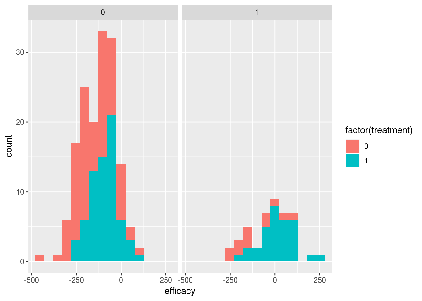
#marginal models
mod0a_code <- "
data {
  int N;
  vector[N] x;
  vector[N] y1;
}
parameters {
  // params for continuous (efficacy) outcome
   vector[2] beta1;
   real<lower=0> sigma;
}
model {
  // marginal for continuous (efficacy) outcome
   vector[N] mu;
   mu = beta1[1] + beta1[2]*x;
   y1 ~ normal(mu, sigma);
}
"

mod0b_code <- "
data {
  int N;
  vector[N] x;
  int<lower=0, upper=1> y2[N];
}
parameters {
  //params for binary (safety) outcome
   vector[2] beta2;
}
model {
  // marginal for binary (safety) outcome
  vector[N] p;
  p = beta2[1] + beta2[2]*x;
  y2 ~ bernoulli(Phi(p));

//    for(i in 1:N){
//      p[i] = normal_cdf(beta2[1] + beta2[2]*x[i], 0, 1);
//      y2[i] ~ bernoulli(p[i]);
//    }

}
"
if (0){
options(mc.cores = parallel::detectCores())
mod0_data <- list(N=nrow(dat), x=dat$treatment, y1=dat$efficacy, y2=dat$safety)
# efficacy marginal model
fit0a <- stan(model_code = mod0a_code, data=mod0_data, iter=1000, chains=4)
print(fit0a)
stan_trace(fit0a)
# safety marginal model
fit0b <- stan(model_code = mod0b_code, data=mod0_data, iter=1000, chains=4)
print(fit0b, pars=c("beta2"))
plot(fit0b)
}
# efficacy marginal model MLE
mle1<-summary(lm(efficacy~treatment,data=dat))
mle1$coefficients[,1]## (Intercept) treatment
## -145.81028 88.00645mle1$sigma## [1] 98.67798# safety marginal model MLE
mle2<-glm(safety~treatment,data=dat,family=binomial(link="probit"))
mle2$coefficients## (Intercept) treatment
## -1.174987 0.707288mod1_code <- "
data {
int N;
vector[N] x;
vector[N] y1;
int<lower=0, upper=1> y2[N];
}
parameters {
// params for continuous (efficacy) outcome
vector[2] beta1;
vector<lower=0>[2] s;
//params for binary (safety) outcome
vector[2] beta2;
// copula dependence param
vector<lower=-2, upper=2>[2] omega;
//real<lower=-1, upper=1> theta12;
}
model {
vector[N] mu;
vector[N] sigma;
vector[N] p;
vector[N] theta;
// marginal for continuous (efficacy) outcome
mu = beta1[1] + beta1[2]*x;
sigma = s[1] + s[2]*x;
// marginal for binary (safety) outcome
p = Phi(beta2[1] + beta2[2]*x);
// copula dependence param
theta = omega[1]+omega[2]*x;
for(i in 1:N){
if (y2[i]==0) {
target += normal_lpdf(y1[i]|mu[i],sigma[i]) + normal_lcdf((inv_Phi(1-p[i])-theta[i]*inv_Phi(normal_cdf(y1[i],mu[i],sigma[i])))/sqrt(1-theta[i]^2)|0,1);
} else {
target += normal_lpdf(y1[i]|mu[i],sigma[i]) + normal_lccdf((inv_Phi(1-p[i])-theta[i]*inv_Phi(normal_cdf(y1[i],mu[i],sigma[i])))/sqrt(1-theta[i]^2)|0,1);
}
}
}
generated quantities {
vector[2] mu;
vector[2] p;
vector[2] theta;
vector[2] rho;
mu[1] = beta1[1];
mu[2] = beta1[1] + beta1[2];
p[1] = Phi(beta2[1]);
p[2] = Phi(beta2[1] + beta2[2]);
theta[1] = omega[1];
theta[2] = omega[1] + omega[2];
rho[1] = theta[1]*exp(normal_lpdf(inv_Phi(p[1])|0,1))/sqrt(p[1]*(1-p[1]));
rho[2] = theta[2]*exp(normal_lpdf(inv_Phi(p[2])|0,1))/sqrt(p[2]*(1-p[2]));
}
"options(mc.cores = parallel::detectCores())
#initalize margins at jittered MLE estimate
init_list <- list(list(beta1=jitter(mle1$coefficients[,1]), s=jitter(rep(mle1$sigma,2))),
list(beta1=jitter(mle1$coefficients[,1]), s=jitter(rep(mle1$sigma,2))))
mod1_data <- list(N=nrow(dat), x=dat$treatment, y1=dat$efficacy, y2=dat$safety)
fit1 <- stan(model_code = mod1_code, data=mod1_data, iter=1000, chains=2, init=init_list)## recompiling to avoid crashing R session## In file included from /home/nathan/R/x86_64-pc-linux-gnu-library/3.4/BH/include/boost/config.hpp:39:0,
## from /home/nathan/R/x86_64-pc-linux-gnu-library/3.4/BH/include/boost/math/tools/config.hpp:13,
## from /home/nathan/R/x86_64-pc-linux-gnu-library/3.4/StanHeaders/include/stan/math/rev/core/var.hpp:7,
## from /home/nathan/R/x86_64-pc-linux-gnu-library/3.4/StanHeaders/include/stan/math/rev/core/gevv_vvv_vari.hpp:5,
## from /home/nathan/R/x86_64-pc-linux-gnu-library/3.4/StanHeaders/include/stan/math/rev/core.hpp:12,
## from /home/nathan/R/x86_64-pc-linux-gnu-library/3.4/StanHeaders/include/stan/math/rev/mat.hpp:4,
## from /home/nathan/R/x86_64-pc-linux-gnu-library/3.4/StanHeaders/include/stan/math.hpp:4,
## from /home/nathan/R/x86_64-pc-linux-gnu-library/3.4/StanHeaders/include/src/stan/model/model_header.hpp:4,
## from file694c1eb82e76.cpp:8:
## /home/nathan/R/x86_64-pc-linux-gnu-library/3.4/BH/include/boost/config/compiler/gcc.hpp:186:0: warning: "BOOST_NO_CXX11_RVALUE_REFERENCES" redefined
## # define BOOST_NO_CXX11_RVALUE_REFERENCES
## ^
## <command-line>:0:0: note: this is the location of the previous definitionprint(fit1, pars=c("mu","p","rho","theta"))## Inference for Stan model: e97bcf4cfd4084814af033552143aa28.
## 2 chains, each with iter=1000; warmup=500; thin=1;
## post-warmup draws per chain=500, total post-warmup draws=1000.
##
## mean se_mean sd 2.5% 25% 50% 75% 97.5%
## mu[1] -146.01 0.32 9.29 -164.10 -152.19 -146.13 -139.81 -127.45
## mu[2] -57.90 0.33 10.41 -77.32 -64.85 -58.08 -51.03 -37.25
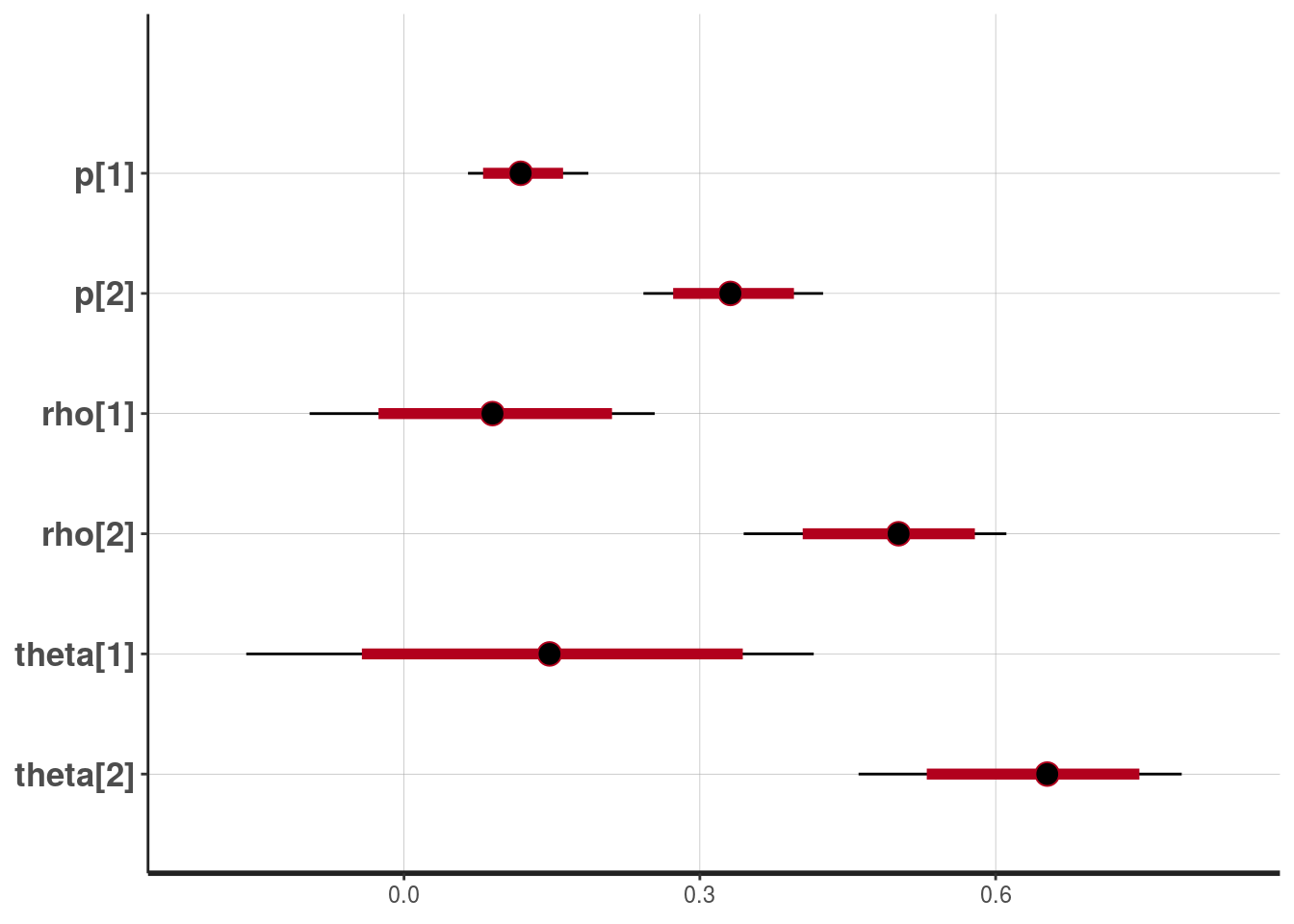
## p[1] 0.12 0.00 0.03 0.06 0.10 0.12 0.14 0.19
## p[2] 0.33 0.00 0.05 0.24 0.30 0.33 0.37 0.43
## rho[1] 0.09 0.00 0.09 -0.10 0.03 0.09 0.15 0.25
## rho[2] 0.50 0.00 0.07 0.34 0.45 0.50 0.54 0.61
## theta[1] 0.15 0.01 0.15 -0.16 0.05 0.15 0.24 0.42
## theta[2] 0.64 0.00 0.09 0.46 0.59 0.65 0.70 0.79
## n_eff Rhat
## mu[1] 858 1.00
## mu[2] 1000 1.00
## p[1] 764 1.00
## p[2] 1000 1.00
## rho[1] 709 1.01
## rho[2] 1000 1.00
## theta[1] 717 1.01
## theta[2] 1000 1.00
##
## Samples were drawn using NUTS(diag_e) at Fri Jan 11 19:13:28 2019.
## For each parameter, n_eff is a crude measure of effective sample size,
## and Rhat is the potential scale reduction factor on split chains (at
## convergence, Rhat=1).stan_trace(fit1, pars=c("mu","p","rho","theta"))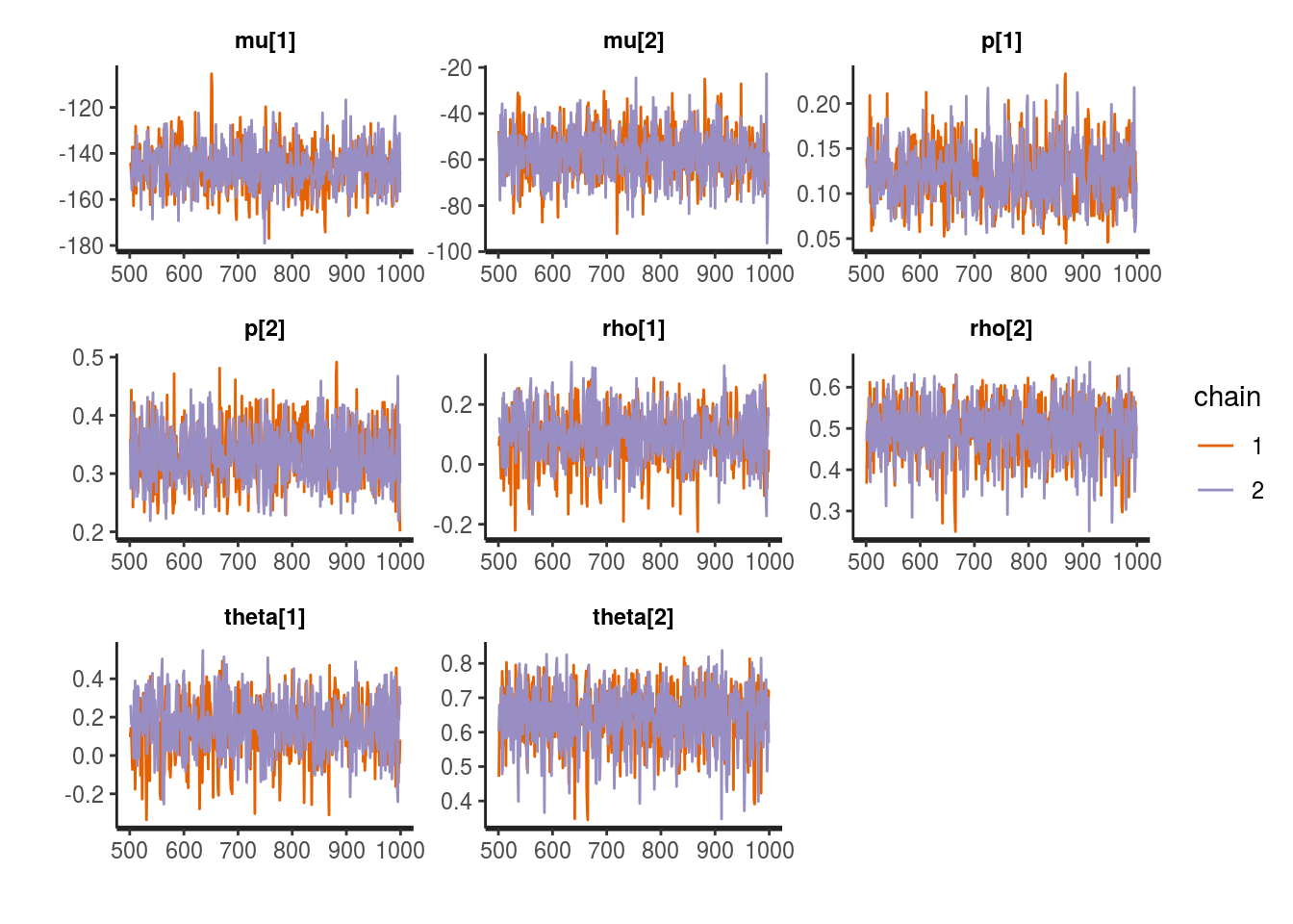
plot(fit1, pars=c("mu"))## ci_level: 0.8 (80% intervals)## outer_level: 0.95 (95% intervals)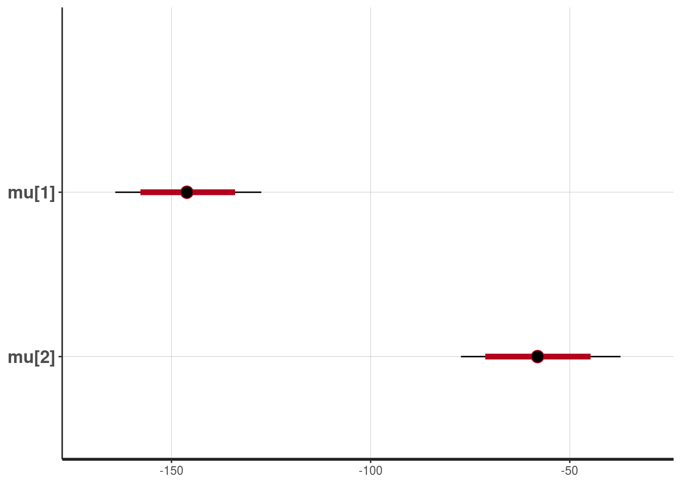
plot(fit1, pars=c("p","rho","theta"))## ci_level: 0.8 (80% intervals)
## outer_level: 0.95 (95% intervals)