copula package
# load packages
libs<-c("copula","scatterplot3d")
invisible(lapply(libs, library, character.only = TRUE))
Elliptical and Archimedean copulas can be defined using the copula class.
Elliptical Copulas
First, we create a normalCopula object with 2 dimensions and (exchangeable) correlation of \(\rho=0.4\)
set.seed(1)

# create normalCopula object with 2 dimensions and exchangeable correlation
myCop.norm <- ellipCopula(family="normal", dim=2, dispstr="ex", param = 0.4)

# generate random draws from copula
u <- rCopula(1000, myCop.norm)
After generating \(n=1000\) random draws from the Normal copula, we check the correlation and produce a scatter plot of the draws
# check correlation
cor(u)
## [,1] [,2]
## [1,] 1.0000000 0.3995705
## [2,] 0.3995705 1.0000000# scatter plot
plot(u[,1],u[,2], main="1000 draws from Normal copula")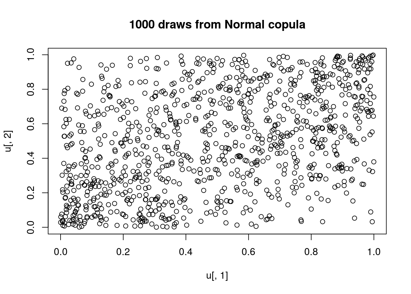
We can also produce contour and perspective plots of the copula density and distribution functions
# contour and perspective plot of density function
contour(myCop.norm,dCopula, main="contour plot of Normal copula density")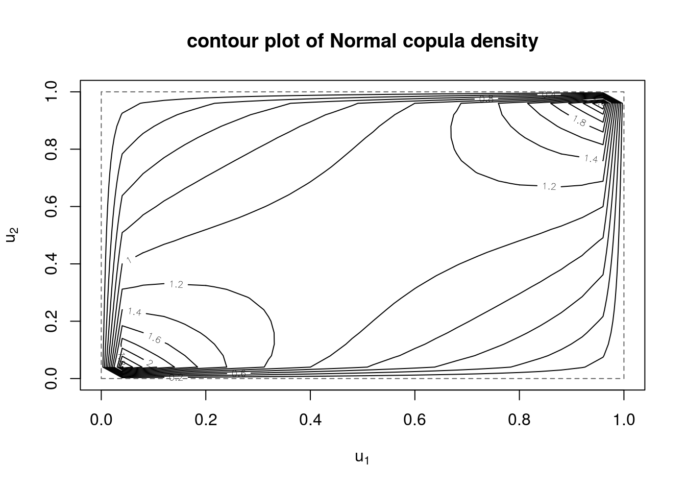
persp(myCop.norm,dCopula, main="perspective plot of Normal copula density")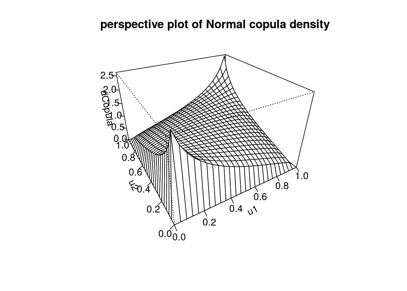
# contour and perspective plot of distribution function
contour(myCop.norm,pCopula, main="contour plot of Normal copula distribution")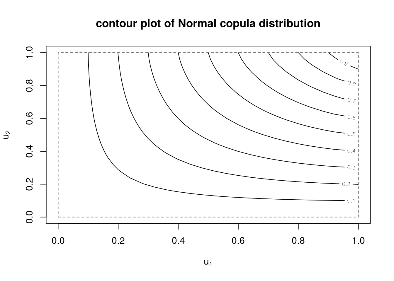
persp(myCop.norm,pCopula, main="perspective plot of Normal copula distribution")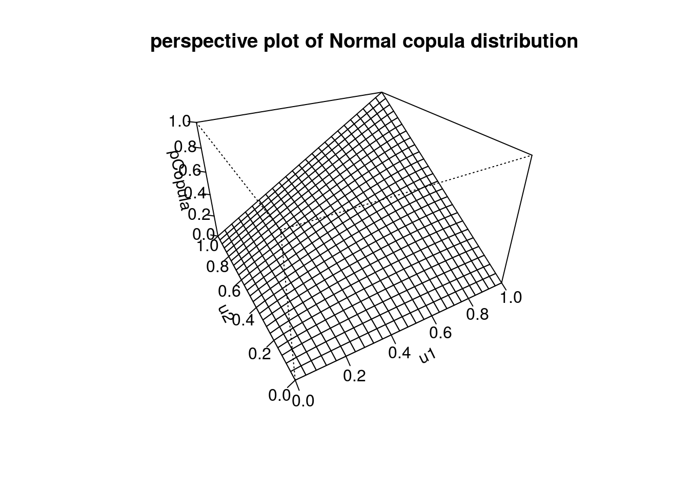
Another common elliptical copula is the \(t\). We create a tCopula model with 8 degrees of freedom and 3 dimensions and specify a banded (Toeplitz) correlation structure with parameters \(\rho_1=0.8\) and \(\rho_2=0.5\).
# create tCopula object with 3 dimensions and banded (toeplitz) correlation and 8 df
myCop.t <- ellipCopula(family="t", dim=3, dispstr="toep", param = c(0.8, 0.5), df=8)
We draw \(n=1000\) samples from this copula and verify that the marginals are uniform and the correlation is correct
v<-rCopula(1000, myCop.t)

par(mfrow=c(1,3), mar=c(2,2,1,1))
hist(v[,1])
hist(v[,2])
hist(v[,3])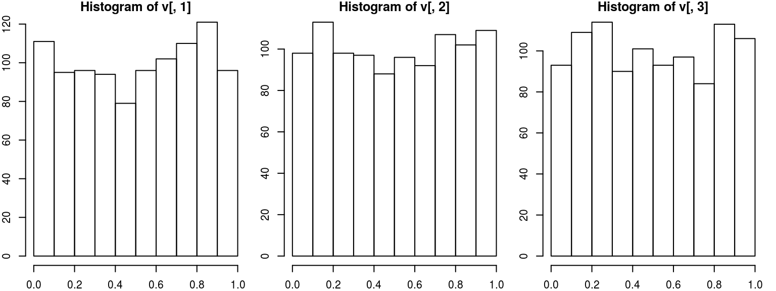
#check correlation
cor(v)
## [,1] [,2] [,3]
## [1,] 1.0000000 0.7963426 0.4895844
## [2,] 0.7963426 1.0000000 0.7870277
## [3,] 0.4895844 0.7870277 1.0000000We can also produce a 3-d scatterplot of a random subset the samples (to avoid overcrowding the plot) and evaluate the copula density and distribution at the sampled values.
# scatter plot
par(mfrow=c(1,1))
subsamp <- sample(1:nrow(v),100)
scatterplot3d(v[subsamp,], type="h")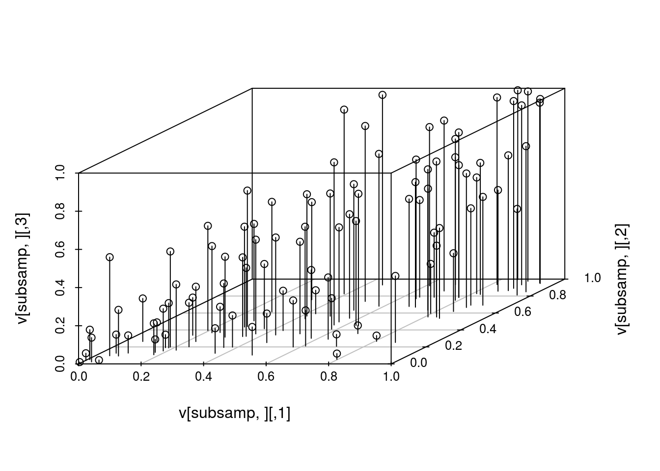
#evaluate density
head(dCopula(v,myCop.t), 10)
## [1] 0.2684407 4.3166171 9.8703657 4.4894340 2.0922633 1.5403350 0.6653583
## [8] 3.5466681 0.2271933 3.1185452#evaluate distribution P(U1 <= u1, U2 <= u2, U3 <= u3)
head(pCopula(v,myCop.t), 10)## [1] 0.01283143 0.67535588 0.02485953 0.11549992 0.58492358 0.19596911
## [7] 0.19517213 0.10670446 0.37418632 0.03529708Archimedean Copulas
Archimedean copulas are another popular choice. We create 3 dimensional Clayton copula with \(\alpha=2\) and a 2 dimensional Frank copula with \(\alpha=5\).
myCop.clayton <- archmCopula(family = "clayton", dim = 3, param = 2)

myCop.frank <- archmCopula(family = "frank", dim = 2, param = 5)
Contour plots for the Frank copula density and distribution are shown below.
par(mfrow=c(1,2))
contour(myCop.frank, dCopula, main="contour plot of Frank copula density", box01=FALSE)
contour(myCop.frank, pCopula, main="contour plot of Frank copula distribution", box01=FALSE)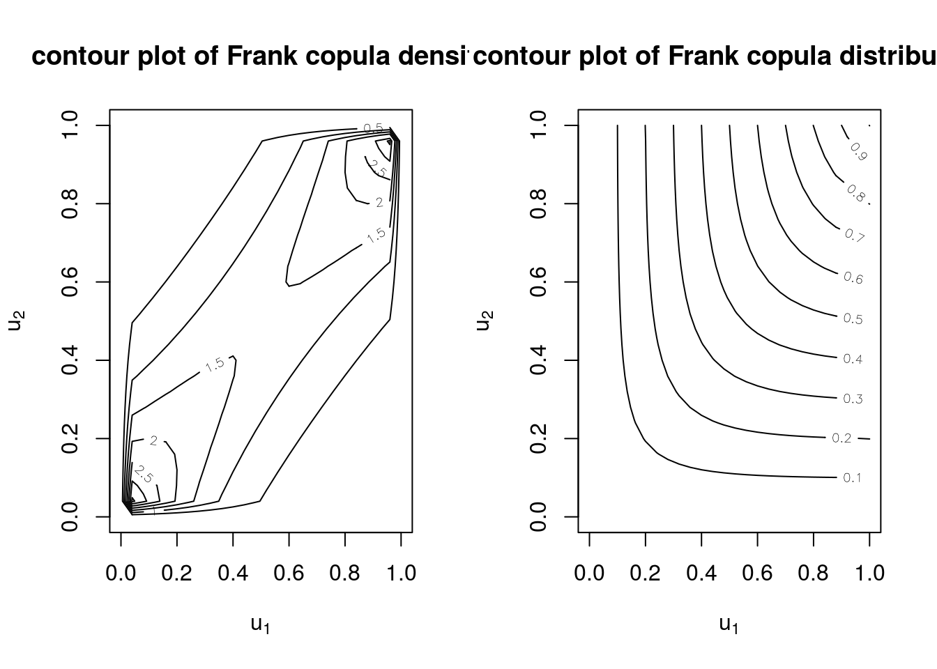
Building multivariate distributions using copulas
Given a copula and marginal distribution functions, the mvdc class defines a multivariate distribution function.
We create a multivariate distribution function by combining 3 normal marginal distributions (\(N(0,2^2)\), \(N(0,1^2)\), and \(N(1,3^2)\)) with a 3-dimensional gumbel copula with \(\alpha=3\). We then draw 1000 samples from this mulivariate distribution and check the marginal means and sds.
myMvd <- mvdc(copula = archmCopula(family="gumbel", dim=3, param=3),
              margins = c("norm", "norm", "norm"),
              paramMargins = list(list(mean=0, sd = 2),
                                  list(mean=0, sd = 1),
                                  list(mean=1, sd = 3)))

# generate random draws from multivariate distribution
w<-rMvdc(1000, myMvd)

# check marginal mean and sd
apply(w,2, function(x) c(mean(x),sd(x)) )
## [,1] [,2] [,3]
## [1,] -0.004235106 0.001274415 0.9862673
## [2,] 1.931454581 0.971024048 2.9104349In addition, we can evaluate the density and distribution at the sampled points
# evaluate density
head(dMvdc(w,myMvd), 10)
## [1] 0.060681635 0.050706591 0.039972322 0.015332861 0.002910626
## [6] 0.011808811 0.031937764 0.022124490 0.007403489 0.012785177# evaluate distribution
head(pMvdc(w,myMvd), 10)## [1] 0.71825269 0.48390858 0.18002531 0.19355349 0.66116464 0.98823123
## [7] 0.69735867 0.56023835 0.33979564 0.09292659Next, we make a 2-dimensional distribution from normal marginals (\(N(0,3)\) and \(N(0,4)\)) and Clayton copula with \(\alpha = 2\) and show the contour and perspective plots of the density and distribution.
myMvd1 <- mvdc(copula = archmCopula(family = "clayton", param = 2),
              margins = c("norm", "norm"),
              paramMargins = list(list(mean=0, sd = 3),
                                  list(mean=0, sd = 4)))

# contour and perspective plots of density
contour(myMvd1, dMvdc, xlim=c(-10,10), ylim=c(-10,10), nlevels=10,
        main="contour plot of 2-d density function\n (Clayton copula, Normal marginals)")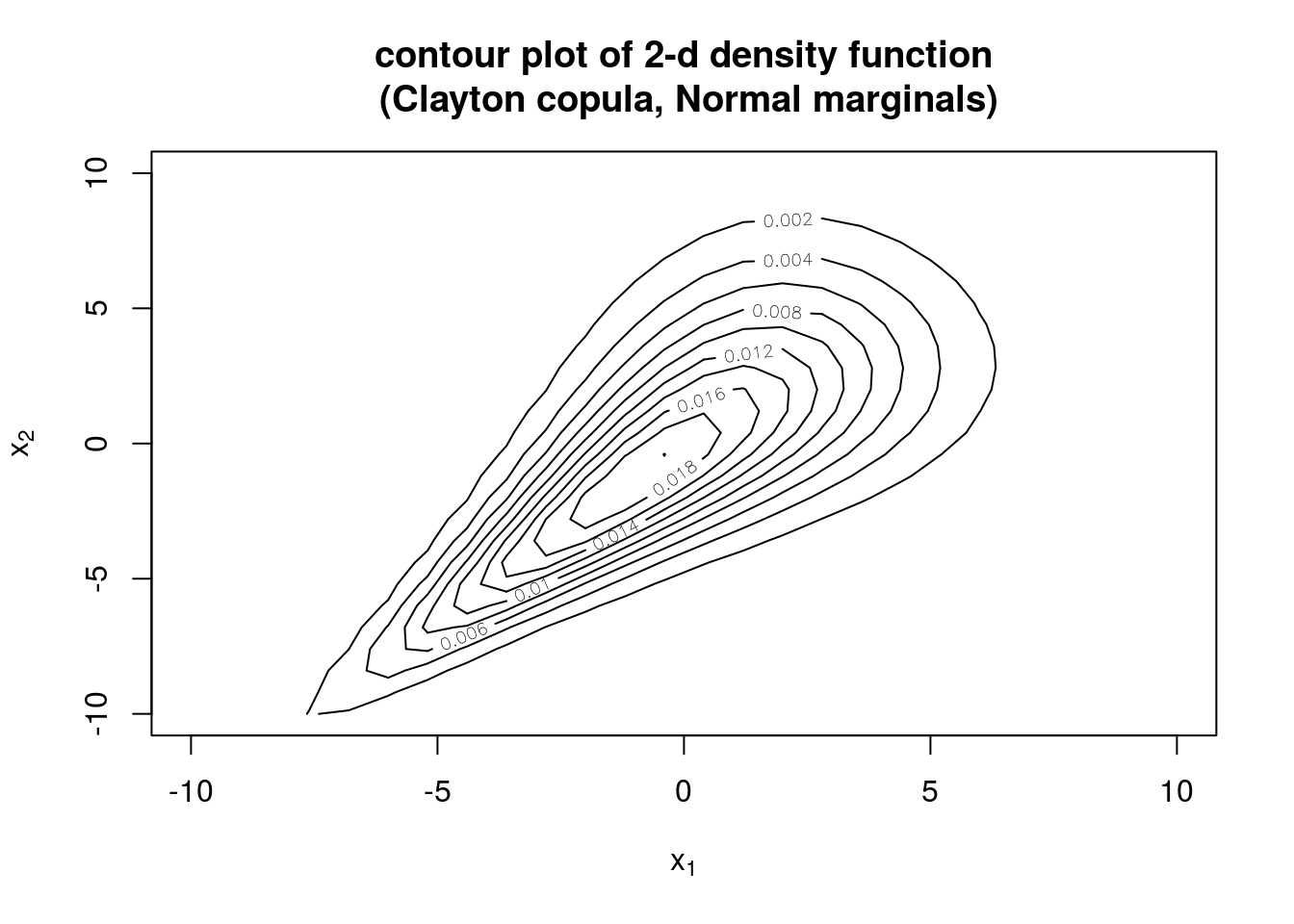
persp(myMvd1, dMvdc, xlim=c(-10,10), ylim=c(-10,10),
      main="perspective plot of 2-d density function\n (Clayton copula, Normal marginals)")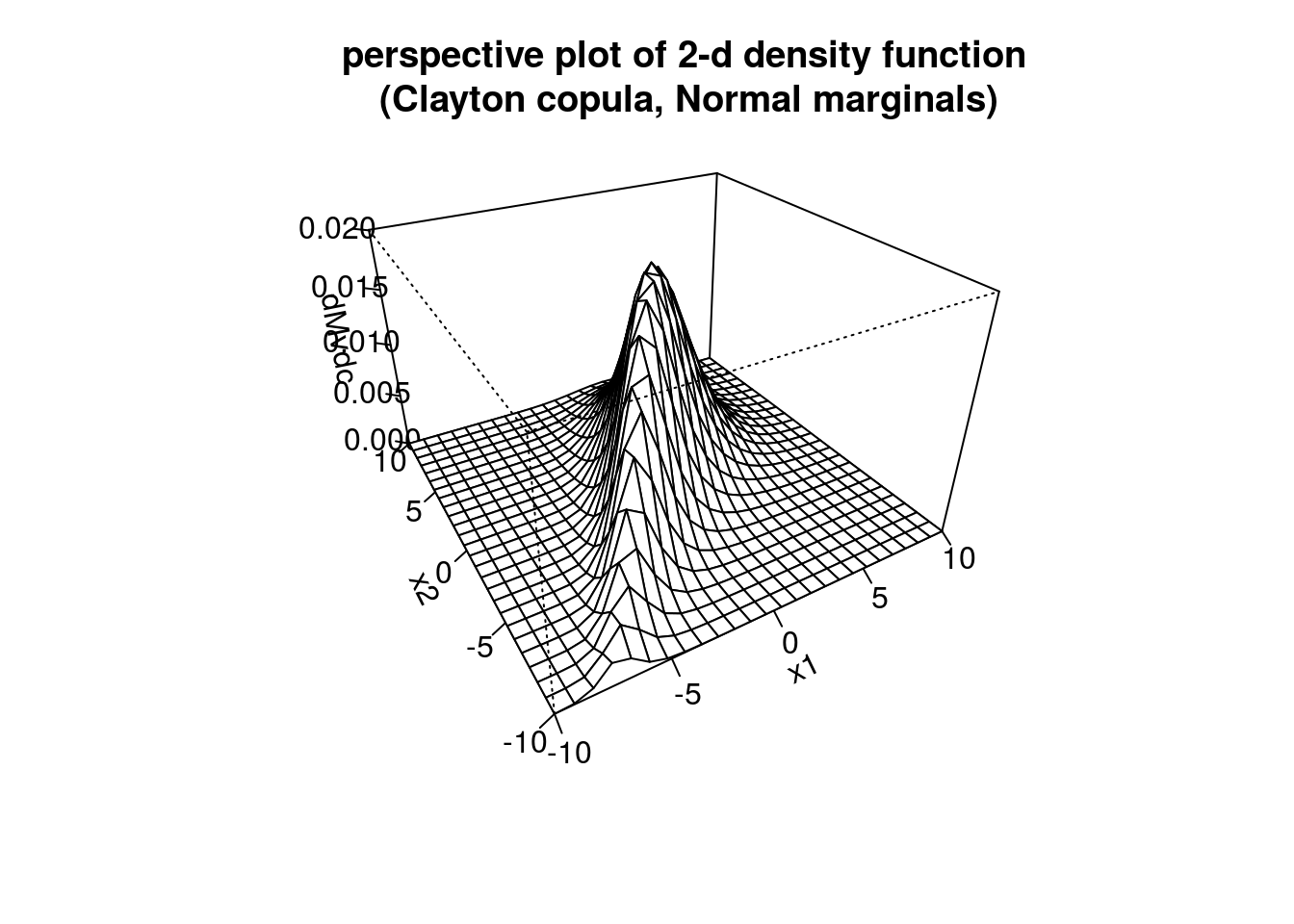
# contour and perspective plots of distribution
contour(myMvd1, pMvdc, xlim=c(-10,10), ylim=c(-10,10), nlevels=10,
        main="contour plot of 2-d distribution function\n (Clayton copula, Normal marginals)")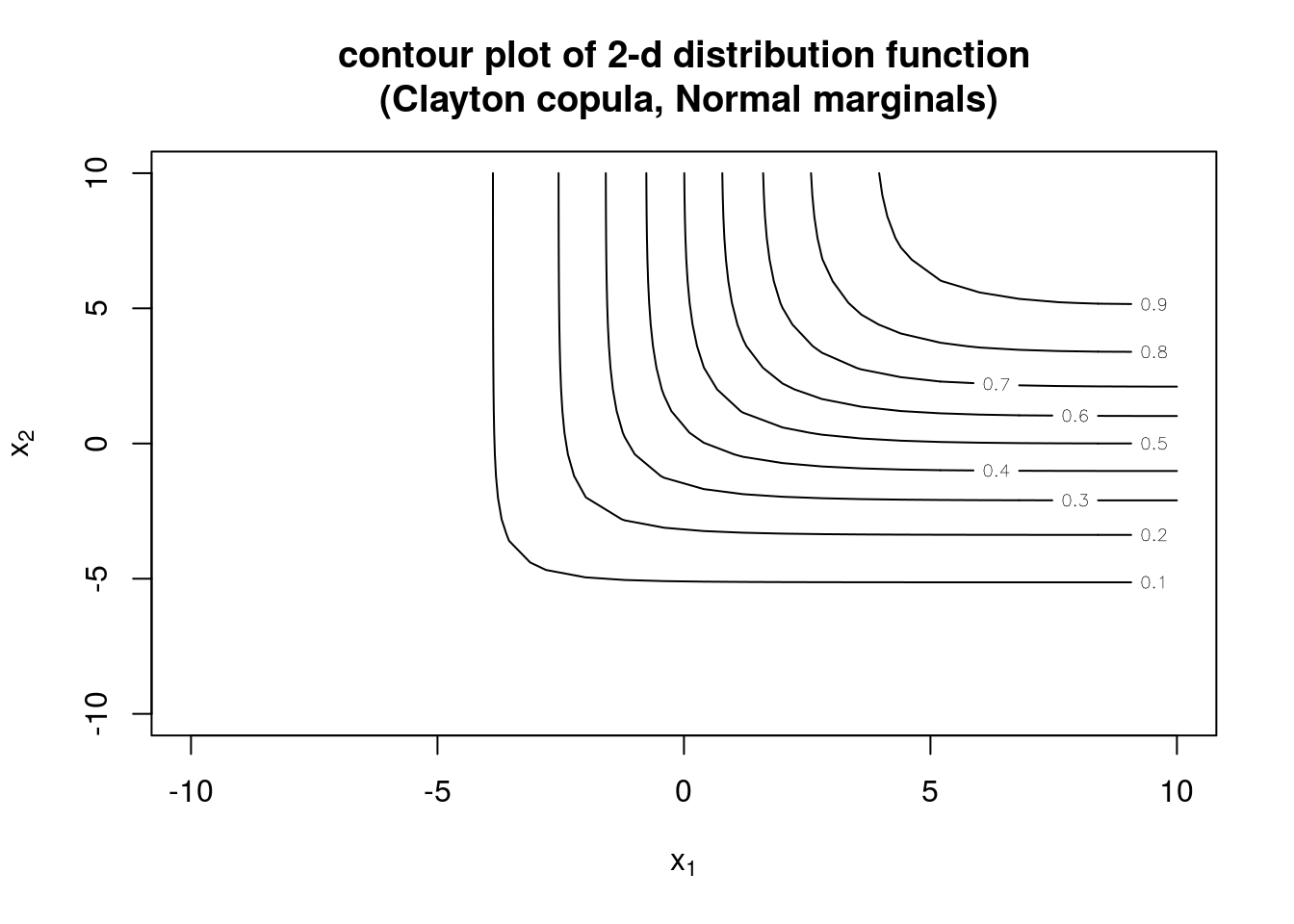
persp(myMvd1, pMvdc, xlim=c(-10,10), ylim=c(-10,10),
      main="perspective plot of 2-d distribution function\n (Clayton copula, Normal marginals)")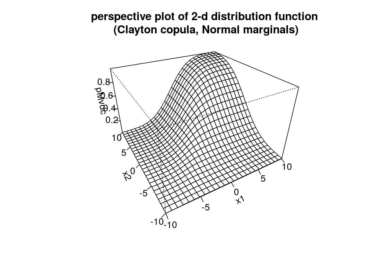
Fitting copula models
The copula package provides the functions loglikCopula() and loglikMvdc() to compute the log-likelihood of the copula and the multivariate copula-based distribution function. fitCopula() and fitMvdc() perform maximum likelihood estimation.
# simulate data
Mvd <- mvdc(copula = ellipCopula(family="normal", param=0.5),
            margins = c("gamma","gamma"),
            paramMargins = list(list(shape=2, scale=1),
                                list(shape=3, scale=2)))
dat <- rMvdc(200, Mvd)

# 'empty' mvdc object, i.e. parameters not specified
Mvd0 <- mvdc(copula = ellipCopula(family="normal"),
            margins = c("gamma","gamma"),
            paramMargins = list(list(shape=NA, scale=NA),
                                list(shape=NA, scale=NA)))

Mvd1 <- mvdc(copula = ellipCopula(family="normal", param=0.8),
            margins = c("gamma","norm"),
            paramMargins = list(list(shape=4, scale=3),
                                list(mean=0, sd=1)))

# loglikelihood w/ correct parameter values
loglikMvdc(c(2,1,3,2,0.5),dat,Mvd)
## [1] -788.8245We calculate the MLEs …
Only the distributional assumptions (form of copula and marginals) of the mvdc class object are used when passed to fitMvdc(); the parameter values from the mvdc object are not used
# method of moments estimates to start optimization
mm <- apply(dat,2,mean)
vv <- apply(dat,2,var)
b1.0 <- c(mm[1]^2/vv[1],vv[1]/mm[1])
b2.0 <- c(mm[2]^2/vv[2],vv[2]/mm[2])
a.0 <- sin(cor(dat[,1], dat[,2], method="kendall")*pi/2)
start <- c(b1.0, b2.0, a.0)

# get MLE
fit <- fitMvdc(dat, Mvd, start = start,
               optim.control = list(trace=TRUE, maxit = 2000))
## initial value 787.745363
## final value 787.113186
## converged
## initial value 787.113186
## final value 787.113186
## stopped after 1 iterationsfit## Call: fitMvdc(data = dat, mvdc = Mvd, start = start, optim.control = list(trace = TRUE,
## maxit = 2000))
## Maximum Likelihood estimation based on 200 2-dimensional observations.
## Copula: normalCopula
## Margin 1 :
## m1.shape m1.scale
## 2.053 1.011
## Margin 2 :
## m2.shape m2.scale
## 3.427 1.713
## Copula:
## rho.1
## 0.4947
## The maximized loglikelihood is -787.1
## Optimization converged# w/ 'empty' mvdc object
fit0 <- fitMvdc(dat, Mvd0, start = start,
optim.control = list(trace=TRUE, maxit = 2000))## initial value 787.745363
## final value 787.113186
## converged
## initial value 787.113186
## final value 787.113186
## stopped after 1 iterationsfit0## Call: fitMvdc(data = dat, mvdc = Mvd0, start = start, optim.control = list(trace = TRUE,
## maxit = 2000))
## Maximum Likelihood estimation based on 200 2-dimensional observations.
## Copula: normalCopula
## Margin 1 :
## m1.shape m1.scale
## 2.053 1.011
## Margin 2 :
## m2.shape m2.scale
## 3.427 1.713
## Copula:
## rho.1
## 0.4947
## The maximized loglikelihood is -787.1
## Optimization converged# misspecified
fit1 <- fitMvdc(dat, Mvd1, start = start,
optim.control = list(trace=TRUE, maxit = 2000))## initial value 1201.877971
## iter 10 value 810.919579
## iter 20 value 800.683656
## iter 20 value 800.683651
## iter 20 value 800.683651
## final value 800.683651
## converged
## initial value 800.683651
## final value 800.683651
## stopped after 1 iterationsfit1## Call: fitMvdc(data = dat, mvdc = Mvd1, start = start, optim.control = list(trace = TRUE,
## maxit = 2000))
## Maximum Likelihood estimation based on 200 2-dimensional observations.
## Copula: normalCopula
## Margin 1 :
## m1.shape m1.scale
## 2.053 1.011
## Margin 2 :
## m2.mean m2.sd
## 5.870 3.034
## Copula:
## rho.1
## 0.4829
## The maximized loglikelihood is -800.7
## Optimization convergedFor large \(p\), we can use an alternative two-stage strategy called inference functions for margins (IFM). In step one IFM estimates the marginal parameters, \(\beta\). In step two, estimates of the copula association parameters \(\alpha\) given \(\hat{\beta}\) are produced. Also called two-stage parametric ML method in censored data setting Note that the SE of \(\hat{\alpha}\) is an underestimate since the variability in \(\hat{\beta}\) is not corectly accounted for.
We can obtain a consistent estimate of \(\alpha\) using canonical ML (CML) which uses the empirical CDFs of each marginal to transform the observations into pseudo-observations. The pseudo-observations are used to estimate \(\hat{\alpha}_{CML}\)
TO incorporate covariates into the margins, we need the log-likelihood function which is the summation of the copula log-likelihood and the log-likelihood of all marginals
(ref equation 9)
# example from appendix A