Chp 2 Definitions and Basic Properties
# load packages
libs<-c("copBasic","lattice","rgl","magrittr")
invisible(lapply(libs, library, character.only = TRUE))
# use lattice for wireframe
# use rgl for persp3d, etc
Consider random vars \(X\) and \(Y\) with distributions functions \(F(x)=P(X \le x)\) and \(G(y)=P(Y \le y)\) and joint distribution \(H(x,y)=P(X \le x, Y \le y)\).
For each pair of \((x,y) \in \mathbb{R} \times \mathbb{R}\), we can associate three numbers \(F(x)\), \(G(y)\) and \(H(x,y)\) (each n interval [0,1]).
\((x,y) \rightarrow (F(x),G(y)) \in [0,1] \times [0,1] \rightarrow H(x,y) \in [0,1]\)
The correspondence that assigns the value of the joint df to each ordered pair of values of the individual dfs is a function called a copula.
Need to generalized notion of “nondecreasing” to multivariate functions
Preliminaries
A “2-increasing” function is a two-dimensional analog of a nondecreasing function of one variable.
Notation: \[ \mathbf{R}: \text{ the real line } (-\infty,\infty)\\ \overline{\mathbf{R}}: \text{ the extended real line } [-\infty,\infty]\\ \overline{\mathbf{R}}^2: \text{ the extended real plane } \overline{\mathbf{R}} \times \overline{\mathbf{R}}\\ B = [x_1,x_2] \times [y_1,y_2]: \text{a rectangle in } \overline{\mathbf{R}}^2 \text{ with vertices } (x_1,y_1),(x_1,y_2),(x_2,y_1),(x_2,y_2)\\ \mathbf{I}^2 = \mathbf{I} \times \mathbf{I} = [0,1] \times [0,1]\\ \text{2-place real function }H: \text{function whose domain, } DomH \subset \overline{\mathbf{R}}^2,\\ \text{ and whose range, } RanH \subset \mathbf{R} \]
Definition: Let \(S_1\) and \(S_2\) be nonempty subsets of \(\overline{\mathbf{R}}\) and \(H\) be a 2-place real function s.t. $DomH = S_1 S_2 $. Let \(B = [x_1,x_2] \times [y_1,y_2]\) be a rectangle with verticesin \(DomH\). The \(H-volume\) of \(B\) is: \[ V_{H}(B)=H(x_2,y_2)-H(x_2,y_1)-H(x_1,y_2)+H(x_1,y_1) \] Definition: A 2-place real function \(H\) is \(2-increasing\) (aka quasi-monotone) if \(V_H(B) \ge 0\) for all rectangles \(B\) whose vertices lie in \(DomH\).
“H is 2-increasing” \(\not\Leftrightarrow\) “H is nondecreasingin each argument”
Ex 2.1
#H volume generator function
mk_Hvol<-function(fun=NULL){

  function(x,y){
    fun(x[2],y[2])-fun(x[2],y[1])-fun(x[1],y[2])+fun(x[1],y[1])
  }

}

# make vectorized function
H1<-function(x,y) mapply(function(x,y) max(x,y),x,y)

# create H-volume function
H1_vol<-mk_Hvol(fun=H1)
Let \(H(x,y)=\max(x,y)\) defined on \(\mathbf{I}^2\). H is a nondecreasing function of \(x\) and \(y\), but the H-volume is \(V_{H}(\mathbf{I}^2)=\)-1, so this function is not 2-increasing. See plots 1, 2, and 3
# for plots
x<-y<-seq(0,1,length=50)
z1<-outer(x,y,FUN="H1") #same as outer(x,y,FUN="pmax")

# color scheme
num_col<-100
#color <- heat.colors(num_col)
color <- rev(rainbow(num_col, start = 0/6, end = 4/6))

contour(x,y,z1)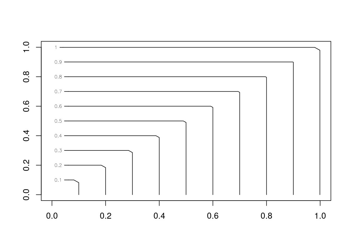
Figure 1: Contour plot
image(x,y,z1,col=color)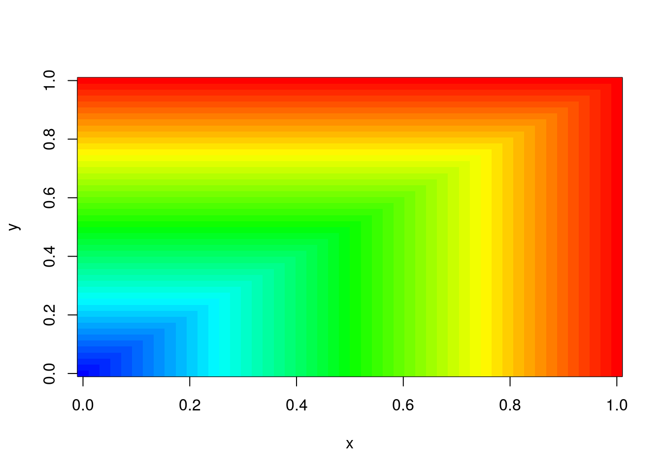
Figure 2: Color image
zcol <- cut(z1, num_col)
plotid1<-persp3d(x,y,z1, col=color[zcol])

fn<-spin3d(axis = c(0, 0, 1), rpm = 6) # spin function

rglwidget(elementId = "plot3drgl1") %>% playwidget(par3dinterpControl(fn, 0, 10, steps=25),
       step = 0.1, loop = TRUE, rate = 0.75)
Figure 3: Interactive
Ex 2.2
# make vectorized function
H2<-function(x,y) mapply(function(x,y) (2*x-1)*(2*y-1), x,y)

# create H-volume function
H2_vol<-mk_Hvol(fun=H2)
Let \(H(x,y)=(2x-1)(2y-1)\) defined on \(\mathbf{I}^2\). \(H\) is 2-increasing since $V_{H}(^2)=$4, but is a decreasing function of \(x\) for each \(y \in (0,1/2)\) and a decreasing function of \(y\) for each \(x\in (0,1/2)\). See plots 4, 5, and 6
z2<-outer(x,y,FUN="H2")
contour(x,y,z2)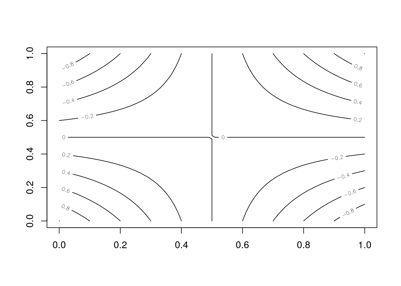
Figure 4: Contour plot
image(x,y,z2,col=color)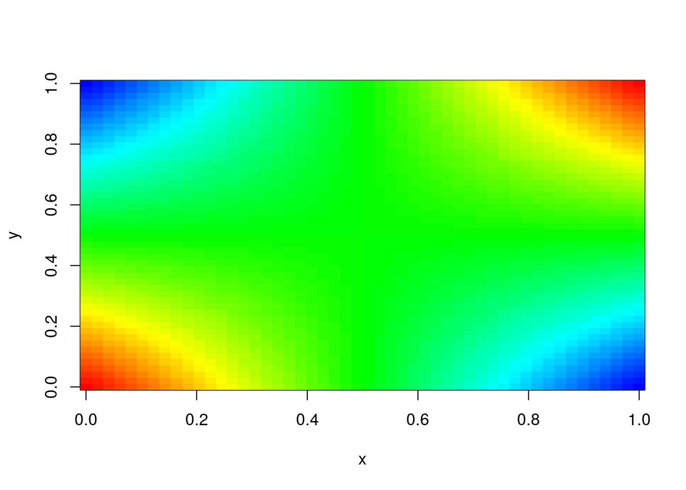
Figure 5: Color Image
z2col  <- cut(z2, num_col)
plotid2 <- persp3d(x,y,z2, col=color[z2col])

rglwidget(elementId = "plot3drgl2") %>% playwidget(par3dinterpControl(fn, 0, 10, steps=25),
       step = 0.1, loop = TRUE, rate = 0.75)
Figure 6: Interactive Plot
Lemma:
Lemma:
Ex 2.3
\(H(x,y)=\frac{(x+1)(e^y-1)}{x+2e^y-1}\)
# make vectorized function
H3<-function(x,y) mapply(function(x,y) ((x+1)*(exp(y)-1))/(x+2*exp(y)-1), x,y)

# create H-volume function
H3_vol<-mk_Hvol(fun=H3)

#check 2-increasing
#H3_vol(c(-1,1),c(1e-15,500))

x3<-seq(-1,1,length=50)
y3<-seq(0,15,length=50)
z3<-outer(x3,y3,FUN="H3")

#H3(x3[4],y3[2])==z3[4,2]contour(x3,y3,z3)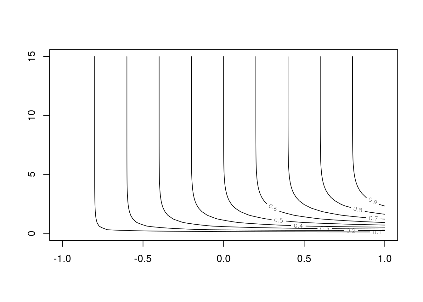
Figure 7: Contour Plot
image(x3,y3,z3,col=color)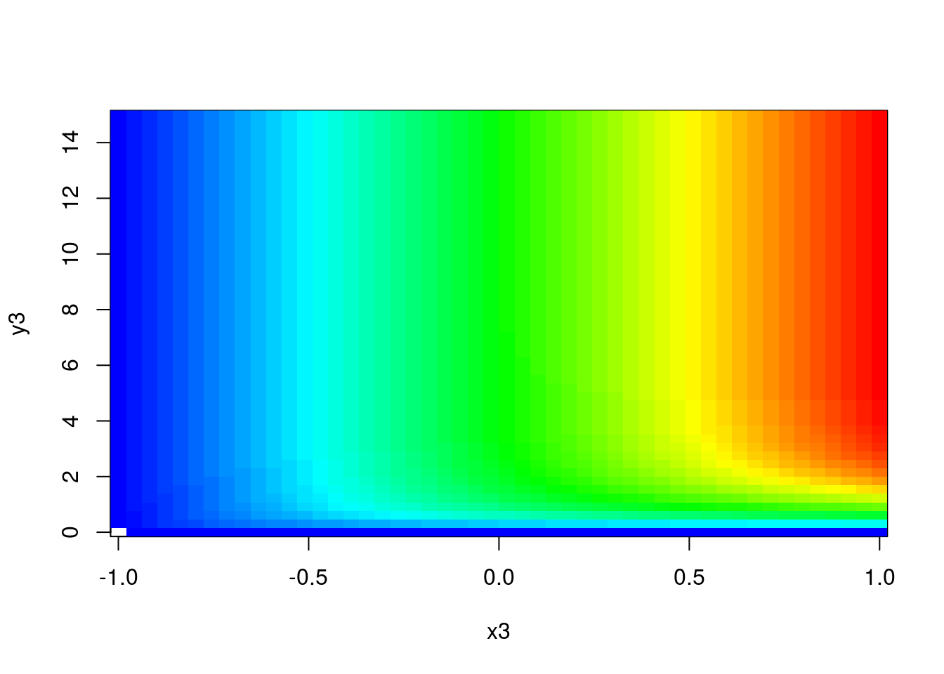
Figure 8: Color Image
z3col  <- cut(z3, num_col)
plotid3<-persp3d(x3,y3,z3, col=color[z3col])

rglwidget(elementId = "plot3drgl3") %>% playwidget(par3dinterpControl(fn, 0, 10, steps=25),  step = 0.1, loop = TRUE, rate = 0.75)
Figure 9: Interactive Plot
Lemma:
Copulas
The graph of any 2-copula is a continuous surface within the unit cube \(\mathbf{I}^3\)which lies between the Fréchet-Hoeffding Bounds
M<-function(u,v) mapply(function(u,v) min(u,v),u,v)
W<-function(u,v) mapply(function(u,v) max(u+v-1,0),u,v)

int01<-seq(0,1,length=50)
mm<-outer(int01,int01,FUN="M")
mmcol <- cut(mm, num_col)

ww<-outer(int01,int01,FUN="W")
wwcol <- cut(ww, num_col)plotid4<-persp3d(int01,int01, mm, col=color[mmcol])
rglwidget(elementId = "plot3drgl4") %>% playwidget(par3dinterpControl(fn, 0, 10, steps=25), step = 0.1, loop = TRUE, rate = 0.75)Figure 10: Frechet-Hoeffding upper bound
plotid5<-persp3d(int01,int01, ww, col=color[wwcol])

rglwidget(elementId = "plot3drgl5") %>% playwidget(par3dinterpControl(fn, 0, 10, steps=25),  step = 0.1, loop = TRUE, rate = 0.75)
Figure 11: Frechet-Hoeffding lower bound
Exercises
Sklar’s Theorem
Definition:
Ex 2.4
Definition:
Ex 2.5
Theorem - Sklar’s Theorem:
Lemma:
Lemma:
Ex 2.6
Definition: